Automotive radar range-Doppler map

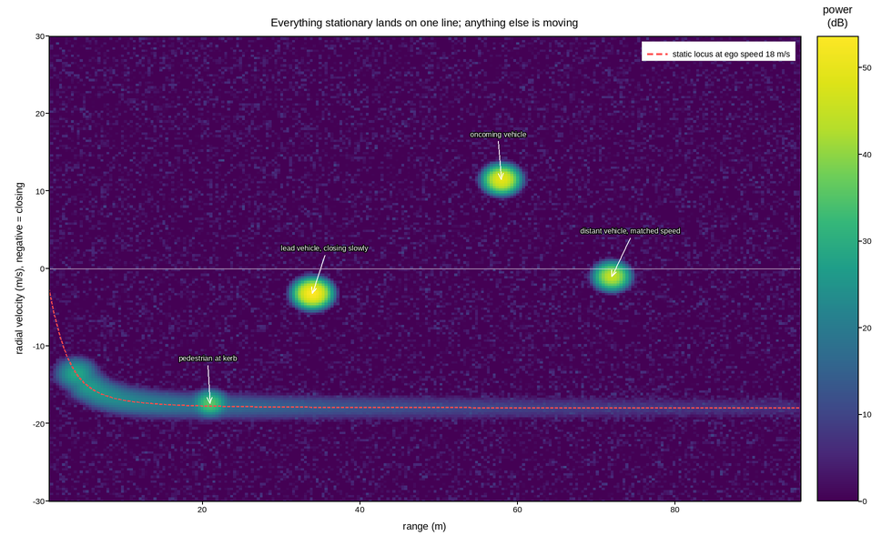
One coherent processing interval from a 77 GHz automotive radar, as the detector sees it: range along one axis, radial velocity along the other, and returned power as the colour. This is the radar’s native coordinate system – the two axes come from two orthogonal FFTs of the same data cube – and reading it directly is how false alarms get understood rather than merely counted.

Power spans about seventy decibels between the guardrail clutter and the weakest pedestrian return, so the mesh carries decibels rather than linear power. That is the domain-standard log transform, and it is applied to the data rather than through a LogNorm because every downstream threshold – detection, constant false alarm rate, tracking – is specified in dB. The colour scale is then floored at the noise level so the map does not spend half its range rendering thermal noise.

The distinctive feature is the diagonal ridge at negative velocity: stationary objects seen from a moving vehicle appear at a radial velocity equal to minus the ego speed times the cosine of the bearing, so the whole static world falls on one predictable locus. Drawing that locus as a line turns “clutter” from a smear into a testable prediction, and every detection off the line is a moving object – which is the discrimination the sensor exists to make.

Live figure — pick a tool, then zoom, pan, point-pick or annotate. Nothing is active until a tool is selected.

View this figure’s Vega export ↗ — the raw JSON spec, rendered live by a real Vega engine.

View this figure’s Vega-Lite export ↗ — the raw JSON spec(s), rendered live by a real Vega-Lite engine.

import numpy as np
import polars as pl
import plotpress

rng = np.random.default_rng(77)

RANGE_BINS, DOPPLER_BINS = 256, 192
MAX_RANGE = 96.0                                   # m
MAX_VELOCITY = 30.0                                # m/s, unambiguous
EGO_SPEED = 18.0                                   # m/s

range_axis = np.linspace(0.5, MAX_RANGE, RANGE_BINS)
velocity_axis = np.linspace(-MAX_VELOCITY, MAX_VELOCITY, DOPPLER_BINS)
R, V = np.meshgrid(range_axis, velocity_axis)

# Thermal noise floor, in linear power.
power = rng.exponential(1.0, R.shape)


def target(r0, v0, rcs, r_width=0.7, v_width=0.55):
    """A point target smeared by the FFT window's mainlobe."""
    return rcs * np.exp(-((R - r0) ** 2) / (2 * r_width ** 2)
                        - ((V - v0) ** 2) / (2 * v_width ** 2))


# Static clutter: guardrail and road furniture, all at -ego speed x cos(bearing).
for r0 in np.arange(4.0, MAX_RANGE, 1.6):
    bearing = np.arctan2(3.5, r0)                  # rail 3.5 m to the side
    power += target(r0, -EGO_SPEED * np.cos(bearing),
                    9.0e3 / r0 ** 1.8, r_width=0.9, v_width=0.7)

TARGETS = [
    (34.0, -3.2, 2.4e5, "lead vehicle, closing slowly"),
    (58.0, 11.5, 9.0e4, "oncoming vehicle"),
    (21.0, -17.4, 4.0e3, "pedestrian at kerb"),
    (72.0, -1.0, 3.0e4, "distant vehicle, matched speed"),
]
for r0, v0, rcs, _ in TARGETS:
    power += target(r0, v0, rcs)

NOISE_FLOOR_DB = 0.0
power_db = 10.0 * np.log10(np.maximum(power, 1e-3))

# One row per range-Doppler bin -- the shape a radar's own data-cube export
# is in, before it is gridded for the mesh.
cube = pl.DataFrame({"range": R.ravel(), "velocity": V.ravel(), "power_db": power_db.ravel()}) \
    .sort(["velocity", "range"])
range_axis = cube["range"].unique().sort().to_numpy()
velocity_axis = cube["velocity"].unique().sort().to_numpy()
power_db = cube["power_db"].to_numpy().reshape(velocity_axis.size, range_axis.size)

fig, ax = plotpress.subplots(figsize=(9.8, 6.0))
mesh = ax.pcolormesh(range_axis, velocity_axis, power_db, cmap="viridis",
                     vmin=NOISE_FLOOR_DB, vmax=float(power_db.max()))
fig.colorbar(mesh, ax=ax).set_title("power\n(dB)")

# The static locus: where everything that is not moving must appear.
bearing = np.arctan2(3.5, range_axis)
ax.plot(range_axis, -EGO_SPEED * np.cos(bearing), color="#ff4d4d",
        linewidth=1.4, linestyle="--",
        label=f"static locus at ego speed {EGO_SPEED:.0f} m/s")

for r0, v0, rcs, name in TARGETS:
    ax.annotate(name, xy=(r0, v0), xytext=(r0 - 4.0, v0 + 5.5),
                arrowprops={"color": "#ffffff"}, color="#ffffff", fontsize=8)

ax.axhline(0.0, color="#ffffff", linestyle=":", linewidth=0.9)
ax.set_xlim(0.5, MAX_RANGE)
ax.set_ylim(-MAX_VELOCITY, MAX_VELOCITY)
ax.set_xlabel("range (m)")
ax.set_ylabel("radial velocity (m/s), negative = closing")
ax.set_title("Everything stationary lands on one line; anything else is moving")
ax.legend(loc="upper right")
fig.tight_layout()