Lidar scan in its native polar coordinates

A single 360-degree sweep from a robot’s laser scanner: range against bearing, plotted on a polar axes because that is the coordinate system the sensor measures in. Converting to Cartesian before plotting is the usual move and it quietly throws away two things worth keeping.

First, the angular sampling is uniform in bearing, not in space, so the points thin out with distance. On a polar plot that is visible and correct; on a Cartesian plot the far wall looks sparse for no stated reason. Second, the maximum range is a property of the sensor, so it is a circle – set_rmax draws the sensor’s horizon as the boundary of the plot rather than as an arbitrary square crop.

Returns that exceed the maximum range are not obstacles at a great distance; they are no return at all, and they must not be plotted as points. They are drawn instead as a light band at the rim, so an open doorway reads as an opening rather than as a wall the sensor happened to miss.

The scan here is a room with a doorway, a pillar and two people. Points are coloured by measured intensity, which distinguishes a retroreflective marker from ordinary wall paint at the same range – the second channel every lidar returns and most plots discard.

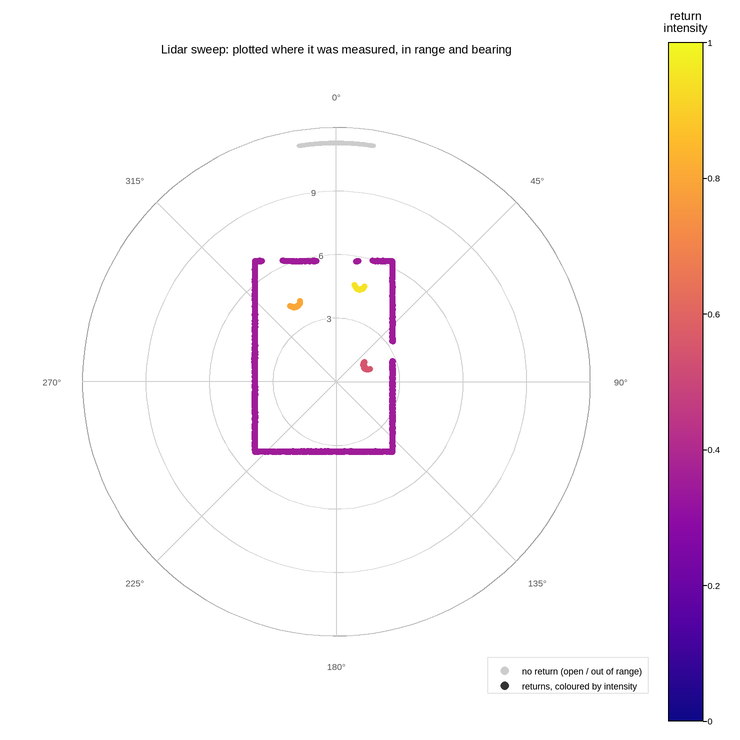
Live figure — pick a tool, then zoom, pan, point-pick or annotate. Nothing is active until a tool is selected.

View this figure’s Vega export ↗ — the raw JSON spec, rendered live by a real Vega engine.

View this figure’s Vega-Lite export ↗ — the raw JSON spec(s), rendered live by a real Vega-Lite engine.

import numpy as np
import polars as pl
import plotpress

rng = np.random.default_rng(360)

N_BEAMS = 1080                                     # 1/3 degree resolution
MAX_RANGE = 12.0                                   # m
bearing = np.linspace(-np.pi, np.pi, N_BEAMS, endpoint=False)

# A rectangular room, 9 m by 6.5 m, with the sensor off-centre.
HALF_X, HALF_Y = 4.5, 3.25
OX, OY = -1.2, 0.6                                 # sensor position in the room

cos_b, sin_b = np.cos(bearing), np.sin(bearing)
with np.errstate(divide="ignore", invalid="ignore"):
    walls = np.minimum(
        np.where(cos_b > 0, (HALF_X - OX) / cos_b, (-HALF_X - OX) / cos_b),
        np.where(sin_b > 0, (HALF_Y - OY) / sin_b, (-HALF_Y - OY) / sin_b),
    )
walls = np.abs(walls)
distance = walls.copy()
intensity = np.full(N_BEAMS, 0.35)


def occlude(centre_x, centre_y, radius, reflectivity):
    """Ray-circle intersection: nearer surfaces win."""
    dx, dy = centre_x - OX, centre_y - OY
    along = dx * cos_b + dy * sin_b
    perp2 = dx ** 2 + dy ** 2 - along ** 2
    hit = (along > 0) & (perp2 < radius ** 2)
    hit_range = along - np.sqrt(np.clip(radius ** 2 - perp2, 0.0, None))
    nearer = hit & (hit_range < distance)
    distance[nearer] = hit_range[nearer]
    intensity[nearer] = reflectivity


occlude(2.6, -1.4, 0.28, 0.80)                     # pillar
occlude(-0.4, 2.1, 0.22, 0.55)                     # person
occlude(3.4, 1.7, 0.24, 0.95)                      # person with a reflective vest

# A doorway in the east wall: no return, so those beams report nothing at all.
doorway = (np.abs(bearing) < 0.16)
distance[doorway] = np.inf

distance += rng.normal(0.0, 0.012, N_BEAMS)        # ranging noise

# One row per beam -- the shape a lidar's own scan packet is in, before
# no-return beams are split from genuine returns.
scan = pl.DataFrame({"bearing": bearing, "distance": distance, "intensity": intensity})
scan = scan.with_columns(
    (~pl.col("distance").is_finite() | (pl.col("distance") > MAX_RANGE)).alias("no_return"))
bearing = scan["bearing"].to_numpy()
distance = scan["distance"].to_numpy()
intensity = scan["intensity"].to_numpy()
no_return = scan["no_return"].to_numpy()

fig = plotpress.Figure(figsize=(7.4, 7.4))
ax = fig.add_subplot(projection="polar")

# Orientation first: a polar axes projects each point as it is added, so the
# zero location and direction have to be settled before any data goes in. Here
# that means clockwise from north -- compass convention, which is what a robot's
# bearings are already quoted in.
ax.set_theta_zero_location("N")
ax.set_theta_direction(-1)

# No-return beams: a rim band, not points at max range.
ax.scatter(bearing[no_return], np.full(no_return.sum(), MAX_RANGE * 0.94),
           s=3.0, color="#cccccc", label="no return (open / out of range)")
returns = ax.scatter(bearing[~no_return], distance[~no_return], s=4.0,
                     c=intensity[~no_return], cmap="plasma", vmin=0.0, vmax=1.0,
                     label="returns, coloured by intensity")
fig.colorbar(returns, ax=ax).set_title("return\nintensity")

ax.set_rmax(MAX_RANGE)
ax.set_rticks([3.0, 6.0, 9.0])   # 12 would sit under the rim band
ax.set_title("Lidar sweep: plotted where it was measured, in range and bearing")
ax.legend(loc="lower right")
fig.tight_layout()