Viewing figures

A figure can be viewed in several ways, from a static image to a fully interactive window. Nothing is global – you always view a specific Figure.

At a glance

Surface	How	Interactive?	Needs
Browser (static)	fig.save("f.svg") / "f.png" then open the file	no	–
Browser (interactive)	fig.save("f.html", interactive=True) then open the file	yes	–
Jupyter (inline)	evaluate fig in a cell	static	–
Jupyter (interactive)	fig.show_in_jupyter()	yes	[jupyter]
Native window	fig.show()	yes	[gui]
Qt window / widget	fig.show_qt() or plotpress.qt.PlotPressWidget	yes	[qt]
Other GUI toolkit (wx, Tk, …)	figure_to_image(fig) (static) or fig.to_html() in a web-view widget (interactive)	depends on the widget	the toolkit itself
Embedded	drop fig.to_svg() / fig.to_html() into your own page	optional	–

In a browser

The most portable options are files you double-click:

fig.save("figure.svg")                       # vector, static
fig.save("figure.html", interactive=True)    # full toolbar, self-contained

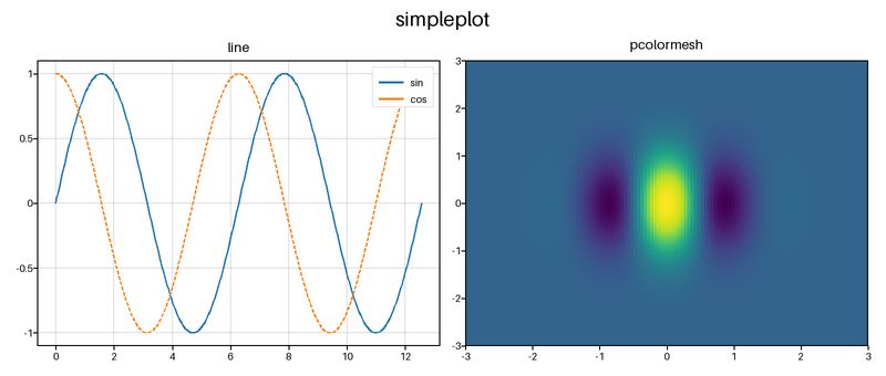
A saved SVG (or PNG) opened in a browser – vector, portable, no toolbar.

The interactive HTML is a single self-contained file (inlined SVG + JS, no external requests), so it opens offline and is easy to share. See Interactive figures for the toolbar.

In Jupyter

Evaluating a figure in a notebook cell displays it inline as static SVG (via Figure._repr_svg_) – crisp, vector, no toolbar:

fig, ax = plotpress.subplots()
ax.plot(x, y)
fig                     # renders inline

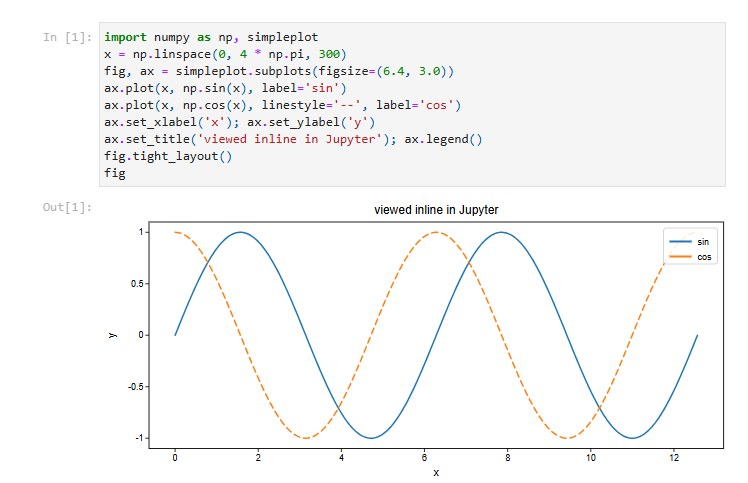
Evaluating fig in a notebook cell renders it inline as static SVG (Figure._repr_svg_).

For the interactive toolbar inside a notebook, use fig.show_in_jupyter() (needs [jupyter]: pip install plotpress[jupyter] – any real Jupyter environment already has IPython). It embeds the same self-contained HTML to_html() produces in an <iframe>, which isolates and runs the inlined JS, so the toolbar, pan/zoom, and point-picking all work exactly as they do in a saved .html file:

fig, ax = plotpress.subplots()
ax.plot(x, y)
fig.show_in_jupyter()   # last expression in the cell, or wrap in display(...)

width/height default to the figure’s own pixel size (figsize x style.dpi) and can be overridden: fig.show_in_jupyter(width=900, height=600).

Under the hood this is just to_html(interactive=True, standalone=False) wrapped in an IPython.display.HTML(...) – standalone=False is meant exactly for embedding in a container you don’t control the size of, so the figure scales to fill the iframe instead of sitting at a fixed pixel size with empty space centered around it. Write that call yourself for more control over the surrounding HTML.

Alternatively, write an .html file and open it, or pop the figure out into a native window with fig.show().

Native window

fig.show() opens the figure in a native OS window (pywebview / WebView2 on Windows, WebKit on macOS, GTK/WebKit on Linux) with the full toolbar. It needs the [gui] extra and blocks until the window is closed; without it, fig.show() falls back to opening the default browser.

fig.show()                               # native window (or browser fallback)
markers = fig.show(wait_for_extract=True) # block, return picked data to Python

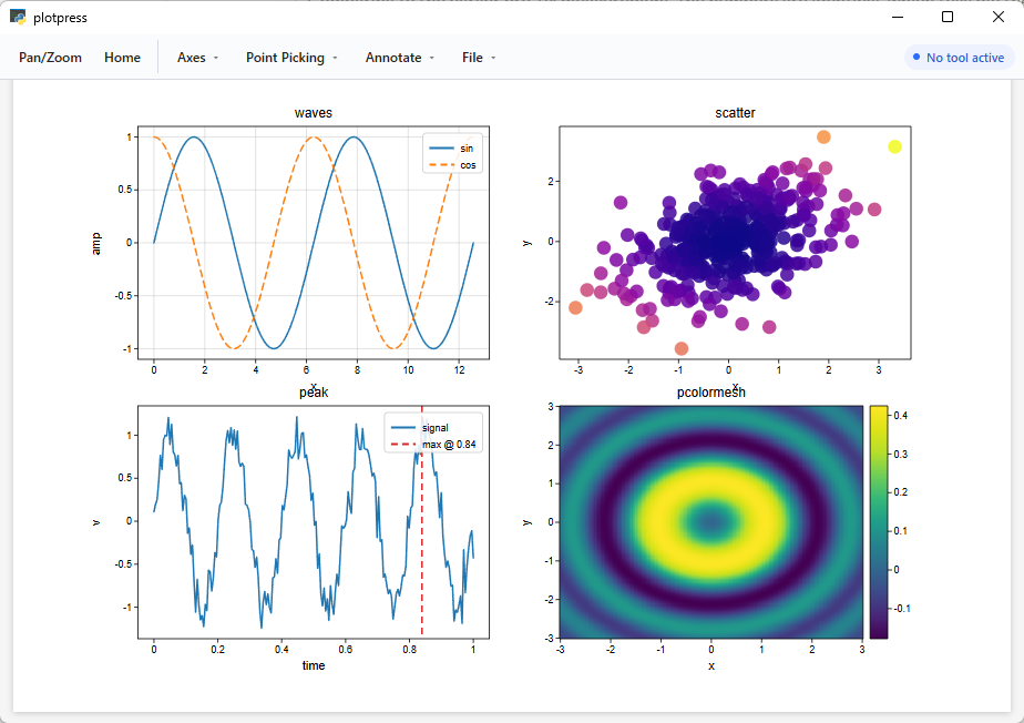
fig.show() – a native OS window hosting the same interactive figure, with the same menu bar (Pan/Zoom, Home, Axes, Point Picking, Annotate, File) as the interactive .html file opened in a browser.

See Saving and showing for wait_for_extract and the extraction format.

In a PyQt / PySide app

For Qt-based desktop apps, plotpress.qt renders the interactive figure in a QWebEngineView – the same toolbar (span / zoom / point-pick / annotate / sliders / extract), reusing the HTML renderer rather than reimplementing it. It works with PyQt6, PySide6, or PyQt5 and needs the [qt] extra (pip install plotpress[qt]).

Quick standalone window:

fig.show_qt()                 # or: import plotpress.qt as spqt; spqt.view(fig)

PlotPressWidget is a plain QWidget, so it embeds into any layout of your own application like any other widget:

from plotpress.qt import PlotPressWidget

plot = PlotPressWidget(fig)          # a QWidget
my_layout.addWidget(plot)             # drop it anywhere

plot.set_figure(other_fig)            # redraw with a different figure
plot.markers(lambda recs: print(recs))  # async: hand picked markers to Python

The widget owns a QWebEngineView (exposed as plot.view for further customization) and loads the document from a temporary file, so even large, mesh-heavy figures render (QWebEngineView.setHtml alone caps at ~2 MB). Pass pick_precision= to shrink the embedded point-pick data for big figures, just as with to_html().

Streaming live data

plot.set_figure(fig) redraws by navigating the QWebEngineView to a fresh page – correct, but that navigation’s own cost (teardown, re-parse, the toolbar JS re-running from scratch) caps updates around 4-5 Hz regardless of how much data is on the figure. For a scope trace, a live sweep, or anything else that needs to redraw many times a second, use plotpress.qt.LiveArtist instead: it loads the figure once, then patches the already-loaded page on every subsequent update rather than reloading it.

from collections import deque
import numpy as np
from plotpress.qt import PlotPressWidget, LiveArtist

fig, ax = plotpress.subplots()
widget = PlotPressWidget()
trace = LiveArtist(widget, fig, ax, color="C0")

xs, ys = deque(maxlen=500), deque(maxlen=500)

def on_new_sample(x, y):
    xs.append(x); ys.append(y)
    trace.update(np.fromiter(xs, float), np.fromiter(ys, float))

A LiveArtist targets one axes on one figure. update() takes the same arguments as the plotting call it wraps – update(x, y) behaves like ax.plot(x, y), update(x, y, C) like ax.pcolormesh(x, y, C) – and any extra keyword arguments passed to the constructor (color, cmap, vmin/vmax, …) are forwarded on every call. A mesh that fills in progressively – the common shape for a real 2-D sweep, most of the grid unmeasured at first – needs no special handling: seed it with NaN and fill cells in as they’re measured, in whatever order they arrive:

mesh = LiveArtist(widget, fig, ax, cmap="viridis", vmin=0, vmax=1)
grid = np.full((ny, nx), np.nan)

def on_new_point(row, col, value):
    grid[row, col] = value
    mesh.update(x_edges, y_edges, grid)

Measured at roughly 55 Hz sustained for a 50,000-point line and 140 Hz for a 100x100 mesh, against the full-reload path’s 4-5 Hz ceiling – a ceiling that doesn’t move with data size, since it comes from the page navigation itself. Point picking stays live too: each update refreshes that axes’ embedded pick data along with the visible SVG (sanitized against NaN/Infinity the same way the initial static payload is), so a click always reports what’s currently on screen rather than data from the first load. The current pan/zoom view and any pins or annotations already on the figure both survive a live update rather than being reset or discarded.

See the live streaming gallery for this pattern applied to specific lab instruments – an oscilloscope, a titration, a raster-scanning microscope, and more.

In other desktop GUI toolkits

plotpress.qt is the one toolkit with a dedicated module, but the two things it does – render a static image, or drop the interactive HTML into a web-view widget – work the same way in any GUI toolkit that has (or can get) one. Two building blocks cover every case:

You want	Call	Gives you
A static image, in memory	plotpress.raster.figure_to_image(fig)	a Pillow Image – .save(buf, format="PNG") for raw bytes, no disk round-trip
The full interactive toolbar	fig.to_html(interactive=True)	a self-contained HTML string – feed it to any web-view widget

A static image needs nothing beyond the toolkit’s own image widget. The interactive toolbar needs a widget that can run JavaScript – typically labelled “web view” or “browser” in each toolkit – and, as with Qt’s QWebEngineView (see above), it is worth loading the HTML from a temp file rather than handing it to an in-memory “set this HTML string” call: several toolkits’ web-view backends silently truncate or choke on large strings, and a mesh-heavy figure’s embedded pick data routinely exceeds that. plotpress.qt does this already; the same pattern is shown for wxPython below.

wxPython

wx.html2.WebView wraps the platform’s native web engine (WebView2 on Windows, WebKit on macOS/GTK) and runs the toolbar’s JS the same way QWebEngineView does:

import os
import tempfile
import wx
import wx.html2

class PlotPanel(wx.Panel):
    def __init__(self, parent, figure):
        super().__init__(parent)
        self.view = wx.html2.WebView.New(self)
        sizer = wx.BoxSizer(wx.VERTICAL)
        sizer.Add(self.view, 1, wx.EXPAND)
        self.SetSizer(sizer)
        self._temp_path = None
        self.set_figure(figure)

    def set_figure(self, figure, interactive=True):
        if self._temp_path:
            try:
                os.remove(self._temp_path)
            except OSError:
                pass
        fd, path = tempfile.mkstemp(suffix=".html", prefix="plotpress_")
        with os.fdopen(fd, "w", encoding="utf-8") as f:
            f.write(figure.to_html(interactive=interactive))
        self._temp_path = path
        self.view.LoadURL("file://" + path)

app = wx.App()
frame = wx.Frame(None, title="plotpress")
panel = PlotPanel(frame, fig)
frame.Show()
app.MainLoop()

For a static (non-interactive) panel instead, skip the web view entirely:

import io
from plotpress.raster import figure_to_image

buf = io.BytesIO()
figure_to_image(fig).save(buf, format="PNG")
bitmap = wx.Bitmap(wx.Image(io.BytesIO(buf.getvalue())))
wx.StaticBitmap(frame, bitmap=bitmap)

Tkinter

Tkinter has no built-in, well-supported web-view widget, so the reliable default is a static image via the standard library’s own PhotoImage (Tk 8.6+ loads PNG directly – no Pillow needed on the Tk side, only to produce the PNG):

import io
import tkinter as tk
from plotpress.raster import figure_to_image

buf = io.BytesIO()
figure_to_image(fig).save(buf, format="PNG")

root = tk.Tk()
photo = tk.PhotoImage(data=buf.getvalue())   # keep a reference -- Tk drops
label = tk.Label(root, image=photo)          # unreferenced PhotoImages
label.pack()
root.mainloop()

For the interactive toolbar, Tkinter’s third-party web-view packages (e.g. tkinterweb) vary in how much of the JS they run – test the toolbar you actually need before relying on one. The simplest option that is guaranteed to run every feature is popping the figure into its own native window from a button callback, using the same webview stack fig.show() already wraps:

button = tk.Button(root, text="Open interactive view", command=fig.show)

Any other toolkit

The same two-tier choice applies everywhere: check whether the toolkit has an embeddable web/browser widget (Kivy, for instance, has third-party kivy_garden webview components); if not, figure_to_image(fig) into whatever image widget it offers is the zero-dependency fallback that always works, at the cost of the toolbar.

Embedded in your own page or app

fig.to_svg() and fig.to_html() return strings, so a figure drops straight into a template, dashboard, report, or web response – no files and no server round-trip:

svg = fig.to_svg()               # inline vector, for reports / emails
page = f"<article>{svg}</article>"

interactive = fig.to_html()      # standalone interactive document