Traffic fundamental diagram

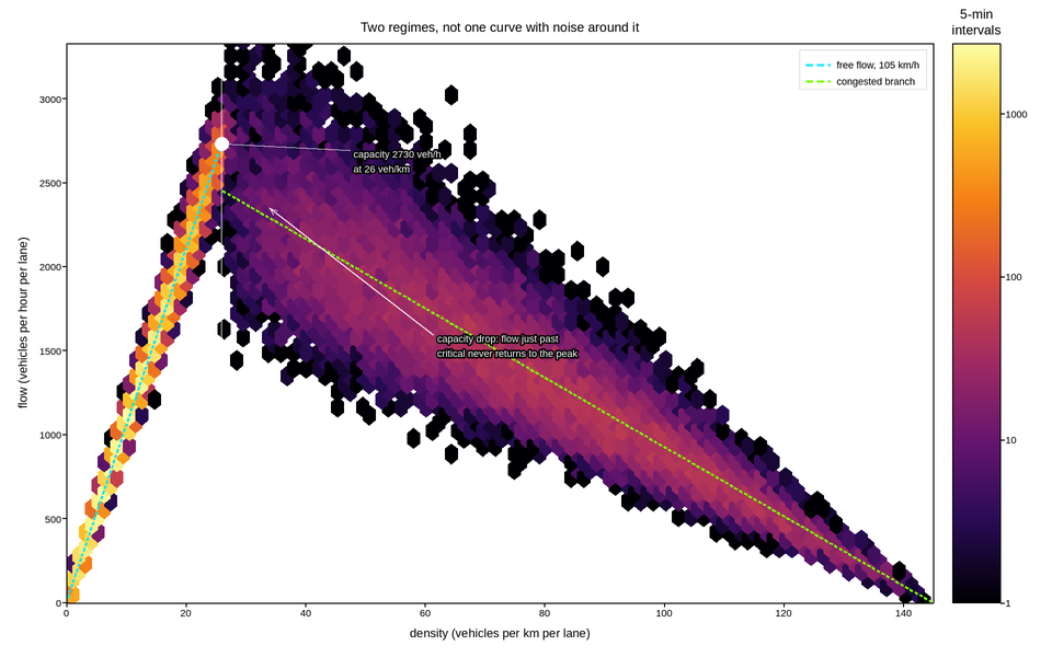
Flow against density from a year of loop-detector records on one motorway lane, one point per five-minute interval. The scatter is not noise around a curve: it is two distinct regimes, and telling them apart is the entire content of traffic flow theory.

Below the critical density traffic is free-flowing and flow rises with density along a tight line whose slope is the free-flow speed. Above it traffic is congested, flow falls as density rises, and the points spread out into a wide cloud because congested traffic is genuinely not a function – the same density supports very different flows depending on how the jam formed.

That spread is why the plot must show the points rather than a fitted curve. About a hundred thousand records need binning, so it is a hexbin with a logarithmic colour scale: the free-flow branch is visited overwhelmingly more often than the congested one, and on a linear count scale the congested branch – the part being studied – is invisible.

Capacity, the peak of the diagram, is marked, and so is the critical density where it occurs. The gap between capacity and the flows actually observed just past it is the capacity drop, a real and much-argued-about effect that this presentation makes visible without needing to be asserted.

Live figure — pick a tool, then zoom, pan, point-pick or annotate. Nothing is active until a tool is selected.

View this figure’s Vega export ↗ — the raw JSON spec, rendered live by a real Vega engine.

View this figure’s Vega-Lite export ↗ — the raw JSON spec(s), rendered live by a real Vega-Lite engine.

import numpy as np
import polars as pl
import plotpress

rng = np.random.default_rng(1935)

FREE_SPEED = 105.0                                 # km/h
JAM_DENSITY = 145.0                                # veh/km
CRITICAL = 26.0                                    # veh/km
CAPACITY = FREE_SPEED * CRITICAL                   # veh/h

N = 105_000
# Most intervals are free-flowing; congestion is the peak-hour minority.
congested = rng.random(N) < 0.18
density = np.where(
    congested,
    CRITICAL + (JAM_DENSITY - CRITICAL) * rng.beta(1.8, 2.6, N),
    CRITICAL * rng.beta(1.6, 2.0, N) * 1.05,
)

flow = np.where(
    congested,
    # Congested branch: wide scatter, and a capacity drop just past critical.
    CAPACITY * 0.90 * (JAM_DENSITY - density) / (JAM_DENSITY - CRITICAL)
    * np.exp(rng.normal(0.0, 0.16, N)),
    density * FREE_SPEED * np.exp(rng.normal(0.0, 0.035, N)),
)
flow = np.clip(flow, 0.0, None)

# One row per five-minute interval -- the shape a loop detector's own record
# export is in, before it is binned into the hexbin.
records = pl.DataFrame({"density": density, "flow": flow})
density = records["density"].to_numpy()
flow = records["flow"].to_numpy()

fig, ax = plotpress.subplots(figsize=(9.6, 6.0))
hb = ax.hexbin(density, flow, gridsize=68, cmap="inferno", mincnt=1,
               norm=plotpress.LogNorm())
fig.colorbar(hb, ax=ax).set_title("5-min\nintervals")

grid = np.linspace(0.0, JAM_DENSITY, 300)
ax.plot(grid[grid <= CRITICAL], grid[grid <= CRITICAL] * FREE_SPEED,
        color="#00e5ff", linewidth=1.8, linestyle="--",
        label=f"free flow, {FREE_SPEED:.0f} km/h")
ax.plot(grid[grid >= CRITICAL],
        CAPACITY * 0.90 * (JAM_DENSITY - grid[grid >= CRITICAL])
        / (JAM_DENSITY - CRITICAL),
        color="#7cff00", linewidth=1.8, linestyle="--", label="congested branch")

ax.axvline(CRITICAL, color="#ffffff", linestyle=":", linewidth=1.3)
ax.scatter([CRITICAL], [CAPACITY], s=9.0, color="#ffffff")
ax.annotate(f"capacity {CAPACITY:.0f} veh/h\nat {CRITICAL:.0f} veh/km",
            xy=(CRITICAL, CAPACITY), xytext=(48.0, 2650.0),
            arrowprops={"color": "#ffffff"}, color="#ffffff", fontsize=9)
ax.annotate("capacity drop: flow just past\ncritical never returns to the peak",
            xy=(34.0, CAPACITY * 0.86), xytext=(62.0, 1550.0),
            arrowprops={"color": "#ffffff"}, color="#ffffff", fontsize=9)

ax.set_xlim(0.0, JAM_DENSITY)
ax.set_ylim(0.0, CAPACITY * 1.22)
ax.set_xlabel("density (vehicles per km per lane)")
ax.set_ylabel("flow (vehicles per hour per lane)")
ax.set_title("Two regimes, not one curve with noise around it")
ax.legend(loc="upper right")
fig.tight_layout()