Drive cycle with speed, acceleration and energy

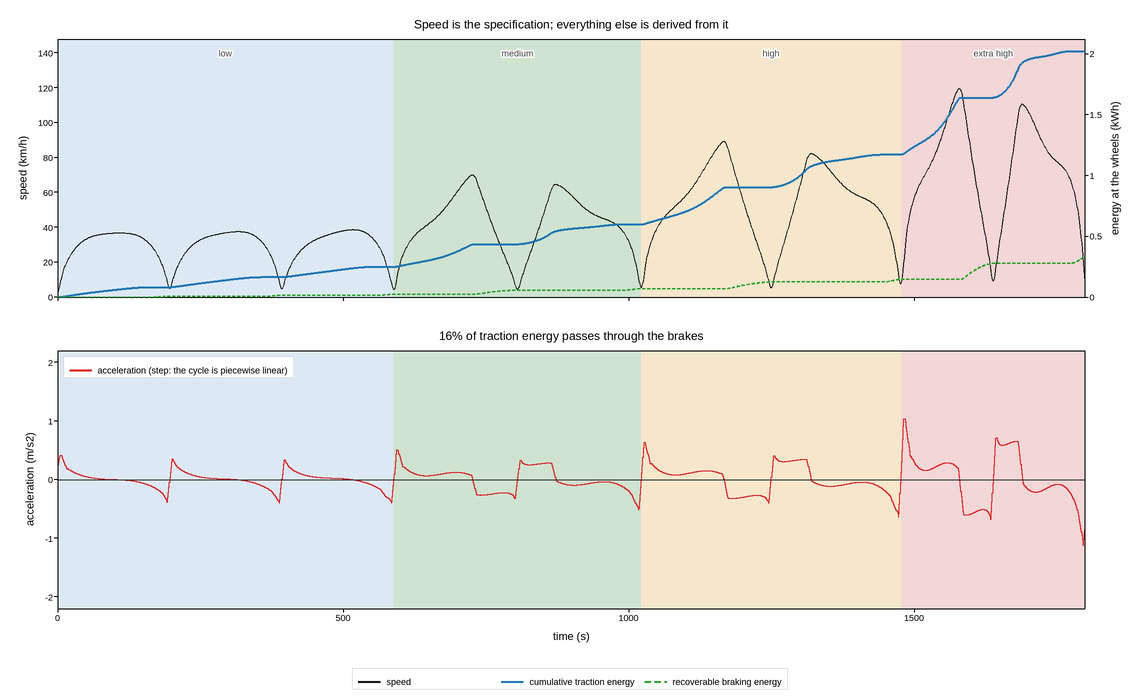
A regulatory drive cycle – the fixed speed-time trace a vehicle is tested against – with the two quantities derived from it that determine what the test actually measures.

Speed is the specification and is drawn on the main axis. Acceleration is its derivative, and the derivative of a piecewise-linear specification is a series of steps, so it is drawn with step rather than plot: the cycle defines constant-acceleration segments, and a smooth line through them would imply a jerk profile the standard does not contain.

Cumulative energy at the wheels goes on a twin axis. It is monotonic and roughly an order of magnitude removed from both other series, and it answers the question the cycle exists to ask – how much work was done – which neither instantaneous series can.

The phases are shaded and named, because a cycle is a concatenation of segments with different purposes: the low-speed urban phases dominate the emissions result while the extra-high-speed phase dominates the energy, and a reader comparing two vehicles needs to know which phase a difference came from. Regenerative braking regions – where acceleration is negative and energy could be recovered – are picked out on the energy trace, since that is where hybrid and conventional drivetrains diverge and the reason the same cycle gives them different answers.

Live figure — pick a tool, then zoom, pan, point-pick or annotate. Nothing is active until a tool is selected.

View this figure’s Vega export ↗ — the raw JSON spec, rendered live by a real Vega engine.

View this figure’s Vega-Lite export ↗ — the raw JSON spec(s), rendered live by a real Vega-Lite engine.

import numpy as np
import polars as pl
import plotpress

# A WLTP-style cycle: (duration, target speed in km/h) segments per phase.
PHASES = [
    ("low", 589, 56.5, "#dce9f5"),
    ("medium", 433, 76.6, "#cfe3d0"),
    ("high", 455, 97.4, "#f6e6cc"),
    ("extra high", 323, 131.3, "#f3d6d6"),
]
MASS = 1520.0                                      # kg
CD_A = 0.68                                        # drag area, m2
RHO = 1.20
CRR = 0.009                                        # rolling resistance

rng = np.random.default_rng(2017)

speed, phase_edges, clock = [], [], 0
for name, duration, peak, _ in PHASES:
    phase_edges.append((clock, clock + duration, name))
    t_local = np.arange(duration)
    # Several accelerate-cruise-decelerate excursions per phase.
    n_cycles = max(2, duration // 190)
    shape = np.abs(np.sin(np.pi * n_cycles * t_local / duration)) ** 0.7
    shape *= 1.0 - 0.35 * np.abs(np.sin(3.1 * np.pi * t_local / duration))
    segment = peak * shape
    segment[:12] = np.linspace(0.0, segment[12], 12)
    speed.append(segment)
    clock += duration

speed = np.concatenate(speed)
speed = np.convolve(speed, np.ones(9) / 9.0, mode="same")   # no infinite jerk
t = np.arange(speed.size, dtype=float)

v = speed / 3.6                                    # m/s
accel = np.gradient(v, t)
force = MASS * accel + 0.5 * RHO * CD_A * v ** 2 + CRR * MASS * 9.81 * (v > 0.1)
power = force * v                                  # W, negative when braking
energy = np.cumsum(np.clip(power, 0.0, None)) / 3.6e6          # kWh, traction only
recoverable = np.cumsum(np.clip(-power, 0.0, None)) / 3.6e6    # kWh at the wheels

# One row per simulation second -- the shape a chassis-dyno logger's own
# trace export is in, before the derived series are plotted from it.
trace = pl.DataFrame({
    "t": t, "speed": speed, "accel": accel, "energy": energy, "recoverable": recoverable,
})
t = trace["t"].to_numpy()
speed = trace["speed"].to_numpy()
accel = trace["accel"].to_numpy()
energy = trace["energy"].to_numpy()
recoverable = trace["recoverable"].to_numpy()

fig, axes = plotpress.subplots(2, 1, figsize=(11.4, 7.0), sharex=True)
ax_v, ax_a = axes

for start, end, name in phase_edges:
    color = dict((p[0], p[3]) for p in PHASES)[name]
    for ax in axes:
        ax.axvspan(start, end, color=color, alpha=1.0)
    ax_v.text(0.5 * (start + end), 138.0, name, ha="center", fontsize=9,
              color="#444444")

ax_v.plot(t, speed, color="#111111", linewidth=1.0, label="speed")
ax_v.set_ylabel("speed (km/h)")
ax_v.set_ylim(0.0, 148.0)
ax_v.set_title("Speed is the specification; everything else is derived from it")

ax_ve = ax_v.twinx()
ax_ve.plot(t, energy, color="#1f77b4", linewidth=1.8,
           label="cumulative traction energy")
ax_ve.plot(t, recoverable, color="#2ca02c", linewidth=1.6, linestyle="--",
           label="recoverable braking energy")
ax_ve.set_ylabel("energy at the wheels (kWh)")
ax_ve.set_ylim(0.0, None)

ax_a.step(t, accel, where="post", color="#d62728", linewidth=0.9,
          label="acceleration (step: the cycle is piecewise linear)")
ax_a.axhline(0.0, color="#333333", linewidth=1.0, linestyle="-")
ax_a.set_xlim(0.0, t[-1])
ax_a.set_ylim(-2.2, 2.2)
ax_a.set_xlabel("time (s)")
ax_a.set_ylabel("acceleration (m/s2)")
ax_a.set_title(f"{recoverable[-1] / energy[-1]:.0%} of traction energy passes "
               "through the brakes")
ax_a.legend(loc="upper left")

fig.legend(ax=[ax_v, ax_ve], loc="lower center", ncol=3)
fig.tight_layout()