C-V measurement and the doping profile extracted from it

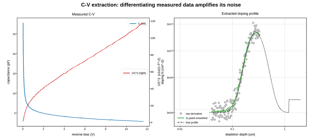
Capacitance-voltage data on the left, and the doping concentration derived from it on the right. The pair is worth drawing together because the derived quantity is what the engineer wants and the raw quantity is where the artefacts live: a bump in the profile is only trustworthy if the capacitance curve is smooth through the same bias.

The extraction is a differentiation. Depletion width comes from the capacitance directly, and doping comes from the slope of 1/C^2 against voltage – which is why 1/C^2 is plotted rather than C. On that axis a uniformly doped sample is a straight line, so a glance says whether the profile is flat before any derivative is taken, and the retrograde implant shows up as a visible bend.

Differentiating measured data amplifies noise, and no amount of plotting hides that. The right panel therefore shows the profile from the raw derivative as faint points and a smoothed version as the line, so the reader can see how much of the structure survives smoothing. Depth spans a decade and concentration spans two, so that panel is log-log; on linear axes the near-surface region – the part a device actually uses – would be compressed into the corner.

Live figure — pick a tool, then zoom, pan, point-pick or annotate. Nothing is active until a tool is selected.

View this figure’s Vega export ↗ — the raw JSON spec, rendered live by a real Vega engine.

View this figure’s Vega-Lite export ↗ — the raw JSON spec(s), rendered live by a real Vega-Lite engine.

import numpy as np
import polars as pl
import plotpress

rng = np.random.default_rng(1247)

Q = 1.602e-19                                      # C
EPS = 11.7 * 8.854e-14                             # F/cm for silicon
AREA = 1.0e-4                                      # cm^2

# A retrograde profile: light at the surface, a buried peak, then the substrate.
depth_ref = np.logspace(-2, 0.3, 400)              # microns
n_ref = (2.0e16
         + 1.4e17 * np.exp(-((np.log10(depth_ref) + 0.55) ** 2) / (2 * 0.16 ** 2))
         + 8.0e15 * (depth_ref > 1.2))

# Forward-model the C-V sweep the profile would produce: integrating the field
# across the depletion region gives the bias that depletes it to each depth.
w = depth_ref * 1e-4                               # cm
bias = np.cumsum(np.gradient(w) * Q * n_ref * w / EPS)
cap = EPS * AREA / w                               # F

keep = (bias > 0.02) & (bias < 12.0)
bias, cap = bias[keep], cap[keep]
cap_meas = cap * (1.0 + rng.normal(0.0, 0.0025, cap.size))   # 0.25% meter noise

# One row per bias step -- the shape an LCR meter's own C-V sweep is in,
# before the doping profile is differentiated from it.
cv_sweep = pl.DataFrame({"bias": bias, "capacitance": cap_meas})
bias = cv_sweep["bias"].to_numpy()
cap_meas = cv_sweep["capacitance"].to_numpy()

inv_c2 = 1.0 / cap_meas ** 2
# N(w) = 2 / (q eps A^2 d(1/C^2)/dV)
slope = np.gradient(inv_c2, bias)
n_raw = 2.0 / (Q * EPS * AREA ** 2 * slope)
depth = EPS * AREA / cap_meas * 1e4                # microns

kernel = np.ones(11) / 11.0
n_smooth = np.convolve(n_raw, kernel, mode="same")
valid = slice(6, -6)                               # drop the convolution edges

fig, axes = plotpress.subplots(1, 2, figsize=(11.0, 4.8))
ax1, ax2 = axes

ax1.plot(bias, cap_meas * 1e12, color="#1f77b4", linewidth=1.8, label="C (left)")
ax1.set_xlabel("reverse bias (V)")
ax1.set_ylabel("capacitance (pF)")
ax1.set_title("Measured C-V")

ax1b = ax1.twinx()
ax1b.plot(bias, inv_c2 / 1e21, color="#d62728", linewidth=1.5,
          label="1/C^2 (right)")
ax1b.set_ylabel("1/C^2  (x1e21 F^-2)")
ax1.legend(loc="upper right")
ax1b.legend(loc="center right")

ax2.scatter(depth[valid], n_raw[valid], s=5.0, color="#bbbbbb",
            label="raw derivative")
ax2.plot(depth[valid], n_smooth[valid], color="#2ca02c", linewidth=2.0,
         label="11-point smoothed")
ax2.plot(depth_ref, n_ref, color="#333333", linestyle="--", linewidth=1.3,
         label="true profile")
ax2.set_xscale("log")
ax2.set_yscale("log")
ax2.set_xlabel("depletion depth (um)")
ax2.set_ylabel("doping N (cm^-3)")
ax2.set_title("Extracted doping profile")
ax2.legend(loc="lower left")
ax2.grid(True)

fig.suptitle("C-V extraction: differentiating measured data amplifies its noise")
fig.tight_layout()