Transfer curve on log and linear axes together

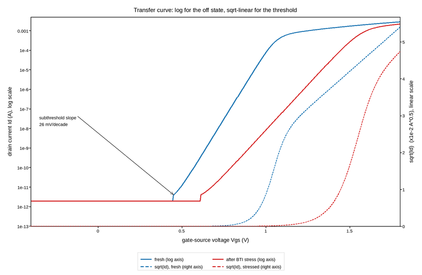
The same transistor sweep plotted twice on one set of axes: drain current on a logarithmic left axis, and the square root of the same current on a linear right axis. This double presentation is the standard way transfer characteristics are reported, because the two axes answer different questions about the same data and neither can answer both.

The log axis covers seven decades, from a picoamp of leakage to a milliamp of drive. Only there is the subthreshold region visible at all, and its slope – millivolts of gate swing per decade of current – is the number that determines how well the device switches off. It is annotated because it is read off the straight portion by construction.

The linear right axis exists for the opposite reason. Above threshold the current is quadratic in gate overdrive, so sqrt(Id) is a straight line whose x-intercept extrapolates to the threshold voltage. That extraction is impossible on the log axis, where everything above threshold is a featureless plateau.

Two devices are shown – a fresh part and one after bias-temperature stress – because the interesting effect is that stress shifts the threshold and degrades the subthreshold slope, and the two changes are only separable when both axes are present.

Live figure — pick a tool, then zoom, pan, point-pick or annotate. Nothing is active until a tool is selected.

View this figure’s Vega export ↗ — the raw JSON spec, rendered live by a real Vega engine.

View this figure’s Vega-Lite export ↗ — the raw JSON spec(s), rendered live by a real Vega-Lite engine.

import numpy as np
import polars as pl
import plotpress

vgs = np.linspace(-0.4, 1.8, 500)

I_OFF = 2.0e-12                                    # junction leakage floor (A)
KT_Q = 0.02585                                     # thermal voltage at 300 K


def transfer(vth, subthreshold_mv_per_decade, beta=1.6e-3):
    """Subthreshold exponential blended into square-law above threshold."""
    n = subthreshold_mv_per_decade / (np.log(10.0) * KT_Q * 1e3)
    weak = I_OFF * np.exp((vgs - vth) / (n * KT_Q))
    strong = beta * np.clip(vgs - vth, 0.0, None) ** 2
    return I_OFF + 1.0 / (1.0 / np.maximum(weak, 1e-30) + 1.0 / np.maximum(strong, 1e-30))


# One row per gate-bias step -- the shape a parameter analyser's own transfer
# sweep is in, before the two devices' curves are drawn on log and sqrt axes.
transfer_sweep = pl.DataFrame({
    "vgs": vgs, "fresh": transfer(0.45, 72.0), "stressed": transfer(0.61, 108.0),
})
vgs = transfer_sweep["vgs"].to_numpy()
fresh = transfer_sweep["fresh"].to_numpy()
stressed = transfer_sweep["stressed"].to_numpy()

fig, ax = plotpress.subplots(figsize=(8.6, 5.6))
ax.plot(vgs, fresh, color="#1f77b4", linewidth=1.8, label="fresh (log axis)")
ax.plot(vgs, stressed, color="#d62728", linewidth=1.8,
        label="after BTI stress (log axis)")
ax.set_yscale("log")
ax.set_ylim(1e-13, 5e-3)
ax.set_ylabel("drain current Id (A), log scale")

ax2 = ax.twinx()
ax2.plot(vgs, np.sqrt(fresh) * 1e2, color="#1f77b4", linestyle="--",
         linewidth=1.4, label="sqrt(Id), fresh (right axis)")
ax2.plot(vgs, np.sqrt(stressed) * 1e2, color="#d62728", linestyle="--",
         linewidth=1.4, label="sqrt(Id), stressed (right axis)")
ax2.set_ylabel("sqrt(Id)  (x1e-2 A^0.5), linear scale")
ax2.set_ylim(0.0, None)

# Subthreshold slope: the steepest part of the log-current curve, which is what
# "mV per decade" means and where a datasheet quotes it from. Reading it off a
# fixed voltage pair instead would land in the leakage floor at low bias, where
# the curve is flat and the number is meaningless.
decades_per_volt = np.gradient(np.log10(fresh), vgs)
steepest = int(np.argmax(decades_per_volt))
slope_mv = 1e3 / decades_per_volt[steepest]
ax.annotate(f"subthreshold slope\n{slope_mv:.0f} mV/decade",
            xy=(vgs[steepest], fresh[steepest]), xytext=(-0.35, 3e-8),
            arrowprops={"color": "#333333"}, fontsize=9)

ax.set_xlim(-0.4, 1.8)
ax.set_xlabel("gate-source voltage Vgs (V)")
ax.set_title("Transfer curve: log for the off state, sqrt-linear for the threshold")
fig.legend(ax=[ax, ax2], loc="lower center", ncol=2)
fig.tight_layout()