Landau-Zener-Stuckelberg interference diamonds

A qubit’s bias is driven sinusoidally through its own avoided crossing, eps(t) = eps0 + A cos(2 pi fd t), sweeping across the tunneling gap twice every drive period instead of once. Each passage is a Landau-Zener transition, and because the passages repeat coherently, the amplitudes from successive passages interfere – the same physics as a Mach-Zehnder interferometer, with time standing in for the second path.

In the weak-tunneling, photon-assisted-tunneling regime the interference resolves into resonances wherever the static detuning matches an integer number of drive quanta, eps0 = n fd, each an n-photon-assisted Landau-Zener transition. Its coupling strength is not fixed but breathes with drive amplitude as J_n(A / fd), the Bessel-function sideband weight from Floquet theory (the same function that sets the ladder brightness in Floquet sideband spectroscopy of a flux-modulated qubit). Every zero of that Bessel function extinguishes its resonance locally, and it is exactly those zeros, threaded across every stripe at once, that carve the characteristic diamond lattice out of an otherwise uniform fan of resonance lines.

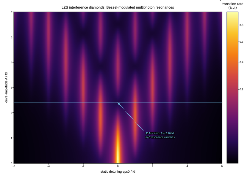
Live figure — pick a tool, then zoom, pan, point-pick or annotate. Nothing is active until a tool is selected.

View this figure’s Vega export ↗ — the raw JSON spec, rendered live by a real Vega engine.

View this figure’s Vega-Lite export ↗ — the raw JSON spec(s), rendered live by a real Vega-Lite engine.

import numpy as np
import polars as pl
import plotpress

FD = 1.0                                           # drive frequency (sets the unit)
LINEWIDTH = 0.12                                    # resonance width, in units of fd
N_SIDEBANDS = 6


def bessel_j(n, x):
    """J_n(x) via its integral representation -- no SciPy for one function.

    ``x`` may be an array; the quadrature axis is kept separate from it.
    """
    theta = np.linspace(0.0, np.pi, 500)
    integrand = np.cos(n * theta[:, None] - x[None, :] * np.sin(theta[:, None]))
    dtheta = theta[1] - theta[0]
    integral = dtheta * (integrand.sum(axis=0) - 0.5 * (integrand[0] + integrand[-1]))
    return integral / np.pi


eps0 = np.linspace(-6.0, 6.0, 340)                  # static detuning, in units of fd
amp = np.linspace(0.0, 6.0, 300)                    # drive amplitude, in units of fd


def lorentzian(detuning, width):
    return width ** 2 / (detuning ** 2 + width ** 2)


# Each n-photon resonance separates into an amplitude-only Bessel weight and
# a detuning-only Lorentzian, so the 2-D response is a sum of outer products
# rather than a full grid evaluation of the Bessel integral.
response_grid = np.zeros((amp.size, eps0.size))
for n in range(-N_SIDEBANDS, N_SIDEBANDS + 1):
    weight = bessel_j(n, amp / FD) ** 2
    response_grid += np.outer(weight, lorentzian(eps0 - n * FD, LINEWIDTH))

EPS0, AMP = np.meshgrid(eps0, amp)

# One row per (detuning, drive amplitude) point -- the shape a swept LZS
# measurement's own output table is in, before it is gridded for the mesh.
result = pl.DataFrame({
    "eps0": EPS0.ravel(), "amp": AMP.ravel(), "response": response_grid.ravel(),
}).sort(["amp", "eps0"])
eps0_axis = result["eps0"].unique().sort().to_numpy()
amp_axis = result["amp"].unique().sort().to_numpy()
response_grid = result["response"].to_numpy().reshape(amp_axis.size, eps0_axis.size)

fig, ax = plotpress.subplots(figsize=(8.4, 6.0))
mesh = ax.pcolormesh(eps0_axis, amp_axis, response_grid, cmap="inferno",
                     norm=plotpress.PowerNorm(0.45))
bar = fig.colorbar(mesh, ax=ax)
bar.set_title("photon-assisted\ntransition rate\n(a.u.)")

# The first Bessel node, J0's first zero, is the sharpest and most recognized
# landmark of the pattern: the n=0 resonance vanishes there while its
# neighbors are still visible.
first_zero = 2.405
ax.axhline(first_zero, color="#7fd8ff", linestyle=":", linewidth=1.0)
ax.annotate(f"J0 first zero, A = {first_zero:.2f} fd:\nn=0 resonance vanishes",
            xy=(0.0, first_zero), xytext=(1.6, 1.15),
            arrowprops={"color": "#7fd8ff"}, color="#7fd8ff", fontsize=9)

ax.set_xlabel("static detuning eps0 / fd")
ax.set_ylabel("drive amplitude A / fd")
ax.set_title("LZS interference diamonds: Bessel-modulated multiphoton resonances")
fig.tight_layout()