Floquet sideband spectroscopy of a flux-modulated qubit

Two-tone spectroscopy of a transmon whose flux is sinusoidally modulated at a fixed drive frequency fd while a weak probe tone sweeps across the band. Continuously modulating the qubit frequency is a periodically driven system in the textbook Floquet sense, and for this particular drive – diagonal in the qubit’s own energy basis – the Floquet theory is exactly solvable rather than merely approximate: the modulated frequency f01(t) = f01_0 + df*cos(2 pi fd t) produces a spectrum with replicas at every f01_0 + n*fd, each weighted by J_n(df/fd)^2, the same Bessel-function sideband weights that describe FM radio and phase-modulated lasers.

That Bessel weighting is the reason the sideband ladder is not uniformly bright. The modulation index beta = df/fd used here sits just past the first zero of J_0, so the carrier itself is strongly suppressed and the brightest lines are the first-order sidebands – a signature that identifies the drive strength directly from which rungs of the ladder light up, without needing to fit anything.

No SciPy dependency is taken for one Bessel function: its integral representation is a five-line trapezoidal quadrature, accurate to numerical noise at this order.

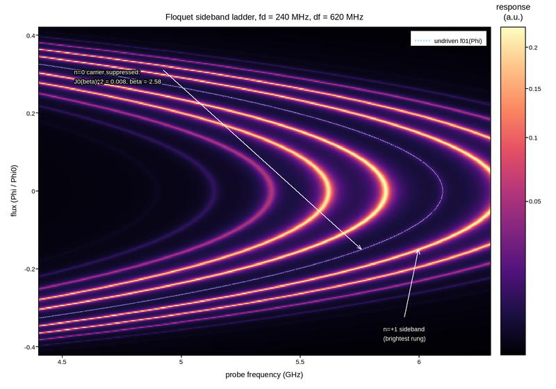
Live figure — pick a tool, then zoom, pan, point-pick or annotate. Nothing is active until a tool is selected.

View this figure’s Vega export ↗ — the raw JSON spec, rendered live by a real Vega engine.

View this figure’s Vega-Lite export ↗ — the raw JSON spec(s), rendered live by a real Vega-Lite engine.

import numpy as np
import polars as pl
import plotpress

F_MAX = 6.10                                       # sweet-spot qubit frequency (GHz)
FD = 0.24                                           # flux modulation frequency (GHz)
DF = 0.62                                           # peak frequency excursion (GHz)
LINEWIDTH = 0.014                                   # probe linewidth (GHz)
N_SIDEBANDS = 6


def bessel_j(n, x):
    """J_n(x) via its integral representation -- no SciPy for one function."""
    theta = np.linspace(0.0, np.pi, 600)
    integrand = np.cos(n * theta - x * np.sin(theta))
    dtheta = theta[1] - theta[0]
    return dtheta * (integrand.sum() - 0.5 * (integrand[0] + integrand[-1])) / np.pi


beta = DF / FD                                      # modulation index
weights = {n: bessel_j(n, beta) ** 2 for n in range(-N_SIDEBANDS, N_SIDEBANDS + 1)}

probe = np.linspace(4.4, 6.3, 420)                  # GHz
flux = np.linspace(-0.42, 0.42, 300)                # Phi / Phi0
P, PHI = np.meshgrid(probe, flux)

f01 = F_MAX * np.sqrt(np.abs(np.cos(np.pi * PHI)))


def lorentzian(detuning, width):
    return width ** 2 / (detuning ** 2 + width ** 2)


response = np.zeros_like(P)
for n, w in weights.items():
    response += w * lorentzian(P - (f01 + n * FD), LINEWIDTH)

# One row per swept (probe frequency, flux) point -- the shape a two-tone
# sweep with the pump left running is actually logged in, before it is
# gridded for the mesh.
sweep = pl.DataFrame({
    "probe_ghz": P.ravel(), "flux_phi0": PHI.ravel(), "response": response.ravel(),
}).sort(["flux_phi0", "probe_ghz"])
probe_axis = sweep["probe_ghz"].unique().sort().to_numpy()
flux_axis = sweep["flux_phi0"].unique().sort().to_numpy()
response = sweep["response"].to_numpy().reshape(flux_axis.size, probe_axis.size)

fig, ax = plotpress.subplots(figsize=(8.0, 5.6))
mesh = ax.pcolormesh(probe_axis, flux_axis, response, cmap="magma",
                     norm=plotpress.PowerNorm(0.5))
bar = fig.colorbar(mesh, ax=ax)
bar.set_title("response\n(a.u.)")

undriven = F_MAX * np.sqrt(np.abs(np.cos(np.pi * flux_axis)))
ax.plot(undriven, flux_axis, color="#7fd8ff", linewidth=0.9, linestyle=":",
        alpha=0.7, label="undriven f01(Phi)")

# Anchor the two annotations to a flux point where both the carrier and its
# first sideband fall inside the probe window, computed from the same
# f01(Phi) used to build the mesh rather than guessed off the rendered image.
flux_anchor = -0.15
f01_anchor = F_MAX * np.sqrt(np.abs(np.cos(np.pi * flux_anchor)))
ax.annotate(f"n=0 carrier suppressed:\nJ0(beta)^2 = {weights[0]:.3f}, beta = {beta:.2f}",
            xy=(f01_anchor, flux_anchor), xytext=(4.55, 0.30),
            arrowprops={"color": "#ffffff"}, color="#ffffff", fontsize=9)
ax.annotate("n=+1 sideband\n(brightest rung)",
            xy=(f01_anchor + FD, flux_anchor), xytext=(5.85, -0.36),
            arrowprops={"color": "#ffffff"}, color="#ffffff", fontsize=9)

ax.set_xlim(probe_axis.min(), probe_axis.max())
ax.set_xlabel("probe frequency (GHz)")
ax.set_ylabel("flux (Phi / Phi0)")
ax.set_title(f"Floquet sideband ladder, fd = {FD * 1e3:.0f} MHz, "
             f"df = {DF * 1e3:.0f} MHz")
ax.legend(loc="upper right")
fig.tight_layout()