Fluxonium level spectrum from exact numerical diagonalization

Fluxonium replaces the transmon’s shunting capacitor-only shunt with a large superinductor, adding a quadratic inductive term to the Josephson potential:

H = 4 EC n^2 + (1/2) EL (phi - phi_ext)^2 - EJ cos(phi)

Because EL is comparable to EJ rather than negligible, the cosine potential is not well approximated by a truncated Taylor series the way a transmon’s is – there is no closed-form spectrum to evaluate. This example diagonalizes the Hamiltonian exactly instead: discretize phi on a grid, build H as a finite-difference matrix, and hand it to numpy.linalg.eigh at every flux point. It is the same technique circuit-QED design software uses, here in about a dozen lines of NumPy.

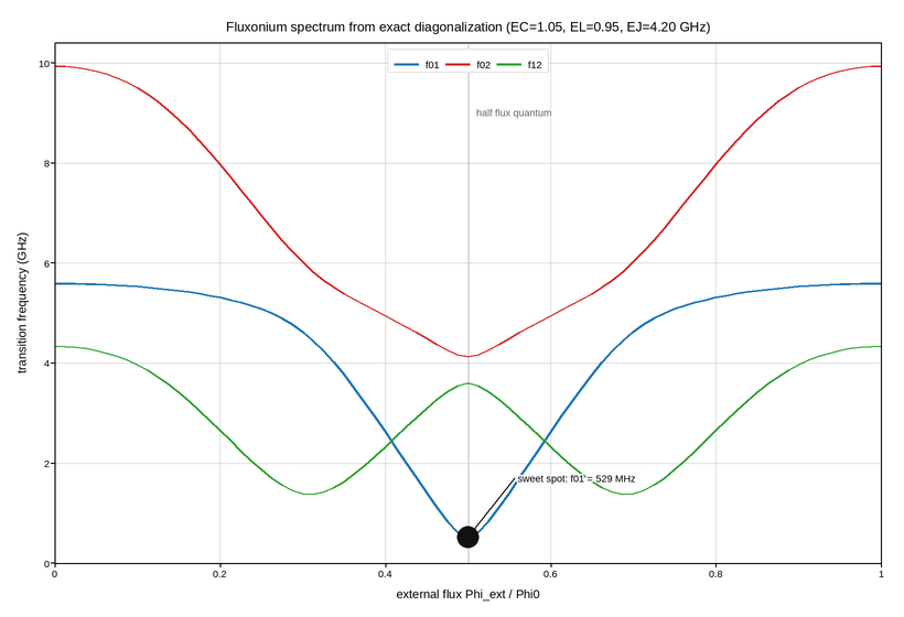
The three lowest transitions are plotted rather than the states themselves. f01 dips to its minimum at half flux quantum, where fluxonium is operated because the qubit is first-order insensitive to flux noise there – the curve is locally flat exactly at the point a transmon’s arch is steepest. f02 stays large everywhere because the second excited state is delocalized across both wells of the double-well potential, and the near-degeneracy of f01 and f12 close to half flux quantum is the qubit’s low anharmonicity at that bias, the price paid for the noise protection.

Live figure — pick a tool, then zoom, pan, point-pick or annotate. Nothing is active until a tool is selected.

View this figure’s Vega export ↗ — the raw JSON spec, rendered live by a real Vega engine.

View this figure’s Vega-Lite export ↗ — the raw JSON spec(s), rendered live by a real Vega-Lite engine.

import numpy as np
import polars as pl
import plotpress

EC = 1.05                                          # charging energy / h (GHz)
EL = 0.95                                          # inductive energy / h (GHz)
EJ = 4.20                                          # Josephson energy / h (GHz)

N_GRID = 360
PHI_SPAN = 4.5 * np.pi                             # grid half-width
phi = np.linspace(-PHI_SPAN, PHI_SPAN, N_GRID)
dphi = phi[1] - phi[0]

# Finite-difference kinetic matrix for -d^2/dphi^2 (tridiagonal, positive
# definite), scaled by 4*EC so H_kin = 4 EC n^2 in the phase basis.
kinetic = np.zeros((N_GRID, N_GRID))
idx = np.arange(N_GRID)
kinetic[idx, idx] = 2.0 / dphi ** 2
kinetic[idx[:-1], idx[:-1] + 1] = -1.0 / dphi ** 2
kinetic[idx[:-1] + 1, idx[:-1]] = -1.0 / dphi ** 2
kinetic *= 4.0 * EC

flux_ext = np.linspace(0.0, 1.0, 81)               # Phi_ext / Phi0
levels = np.zeros((flux_ext.size, 4))
for k, f in enumerate(flux_ext):
    phi_ext = 2.0 * np.pi * f
    potential = 0.5 * EL * (phi - phi_ext) ** 2 - EJ * np.cos(phi)
    h = kinetic.copy()
    h[idx, idx] += potential
    eigenvalues = np.linalg.eigvalsh(h)
    levels[k] = eigenvalues[:4]

# One row per flux point, one column per diagonalized level -- the shape a
# numerical diagonalization's own output table is in, before transition
# frequencies are differenced from it.
spectrum = pl.DataFrame({
    "flux_phi0": flux_ext,
    "e0": levels[:, 0], "e1": levels[:, 1], "e2": levels[:, 2], "e3": levels[:, 3],
})
spectrum = spectrum.with_columns(
    (pl.col("e1") - pl.col("e0")).alias("f01"),
    (pl.col("e2") - pl.col("e0")).alias("f02"),
    (pl.col("e2") - pl.col("e1")).alias("f12"),
)
flux_axis = spectrum["flux_phi0"].to_numpy()
f01 = spectrum["f01"].to_numpy()
f02 = spectrum["f02"].to_numpy()
f12 = spectrum["f12"].to_numpy()

sweet_spot = int(np.argmin(f01))

fig, ax = plotpress.subplots(figsize=(8.2, 5.6))
ax.plot(flux_axis, f01, color="#1f77b4", linewidth=2.0, label="f01")
ax.plot(flux_axis, f02, color="#d62728", linewidth=1.6, label="f02")
ax.plot(flux_axis, f12, color="#2ca02c", linewidth=1.6, label="f12")

ax.axvline(0.5, color="#888888", linestyle=":", linewidth=1.2)
ax.scatter([flux_axis[sweet_spot]], [f01[sweet_spot]], s=14.0, color="#111111")
ax.annotate(f"sweet spot: f01 = {f01[sweet_spot] * 1e3:.0f} MHz",
            xy=(flux_axis[sweet_spot], f01[sweet_spot]),
            xytext=(flux_axis[sweet_spot] + 0.06, f01[sweet_spot] + 1.1),
            arrowprops={"color": "#111111"}, fontsize=9)
ax.text(0.51, f02.max() * 0.9, "half flux quantum", fontsize=9, color="#666666")

ax.set_xlim(0.0, 1.0)
ax.set_ylim(0.0, None)
ax.set_xlabel("external flux Phi_ext / Phi0")
ax.set_ylabel("transition frequency (GHz)")
ax.set_title(f"Fluxonium spectrum from exact diagonalization "
             f"(EC={EC:.2f}, EL={EL:.2f}, EJ={EJ:.2f} GHz)")
ax.legend(loc="upper center", ncol=3)
ax.grid(True)
fig.tight_layout()