Autler-Townes splitting of a probed transition

A three-level ladder – ground |0>, intermediate |1>, and a second excited state |2> – with a strong control field driving |1>-|2> resonantly (or near it) while a weak probe sweeps across |0>-|1>. The control field does not just shift the |1>-|2> transition; it dresses |1> and |2> into two new eigenstates split by the generalized Rabi frequency, and the probe – which only ever sees |1> – reports that splitting as two peaks instead of one. This is the frequency-domain twin of Rabi oscillation: where a time-domain Rabi experiment watches population oscillate, Autler-Townes spectroscopy watches the same coherent coupling split a spectral line.

The dressed-state formula is closed form,

f+- = Dc/2 +- (1/2) sqrt(Omega_c^2 + Dc^2),

with the two peaks carrying weight cos^2(theta) and sin^2(theta) for mixing angle theta = atan2(Omega_c, Dc)/2. At exact control resonance (Dc = 0) the split is symmetric and both peaks carry equal weight; a nonzero control detuning tilts the split and trades intensity between the peaks, which is the fan this example plots against control power.

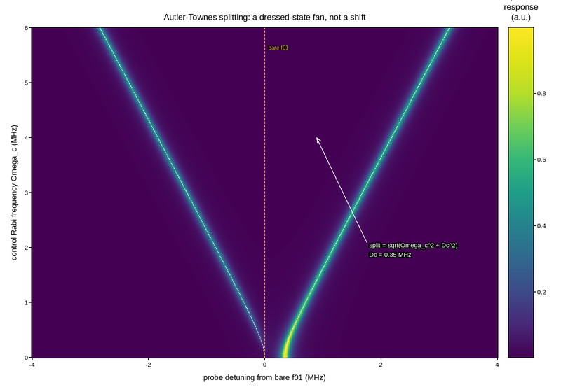
Live figure — pick a tool, then zoom, pan, point-pick or annotate. Nothing is active until a tool is selected.

View this figure’s Vega export ↗ — the raw JSON spec, rendered live by a real Vega engine.

View this figure’s Vega-Lite export ↗ — the raw JSON spec(s), rendered live by a real Vega-Lite engine.

import numpy as np
import polars as pl
import plotpress

CONTROL_DETUNING = 0.35                            # Dc, control detuning (MHz)
LINEWIDTH = 0.06                                    # probe linewidth (MHz)

probe = np.linspace(-4.0, 4.0, 380)                 # MHz, relative to bare f01
rabi_c = np.linspace(0.0, 6.0, 300)                 # control Rabi frequency (MHz)
F, OMEGA = np.meshgrid(probe, rabi_c)

generalized = np.sqrt(OMEGA ** 2 + CONTROL_DETUNING ** 2)
f_plus = 0.5 * CONTROL_DETUNING + 0.5 * generalized
f_minus = 0.5 * CONTROL_DETUNING - 0.5 * generalized

theta = 0.5 * np.arctan2(OMEGA, CONTROL_DETUNING)
weight_plus = np.cos(theta) ** 2
weight_minus = np.sin(theta) ** 2


def lorentzian(detuning, width):
    return width ** 2 / (detuning ** 2 + width ** 2)


response = (weight_plus * lorentzian(F - f_plus, LINEWIDTH)
            + weight_minus * lorentzian(F - f_minus, LINEWIDTH))

# One row per swept (probe frequency, control Rabi frequency) point -- the
# shape a probe-and-control two-tone sweep is actually logged in, before it
# is gridded for the mesh.
sweep = pl.DataFrame({
    "probe_mhz": F.ravel(), "rabi_c_mhz": OMEGA.ravel(), "response": response.ravel(),
}).sort(["rabi_c_mhz", "probe_mhz"])
probe_axis = sweep["probe_mhz"].unique().sort().to_numpy()
rabi_axis = sweep["rabi_c_mhz"].unique().sort().to_numpy()
response_grid = sweep["response"].to_numpy().reshape(rabi_axis.size, probe_axis.size)

fig, ax = plotpress.subplots(figsize=(8.0, 5.6))
mesh = ax.pcolormesh(probe_axis, rabi_axis, response_grid, cmap="viridis")
bar = fig.colorbar(mesh, ax=ax)
bar.set_title("probe\nresponse\n(a.u.)")

branch_omega = np.linspace(0.0, 6.0, 200)
branch_gen = np.sqrt(branch_omega ** 2 + CONTROL_DETUNING ** 2)
ax.plot(0.5 * CONTROL_DETUNING + 0.5 * branch_gen, branch_omega,
        color="#ffffff", linestyle=":", linewidth=1.0)
ax.plot(0.5 * CONTROL_DETUNING - 0.5 * branch_gen, branch_omega,
        color="#ffffff", linestyle=":", linewidth=1.0)

ax.axvline(0.0, color="#ff9d5c", linestyle="--", linewidth=1.0)
ax.text(0.06, 5.6, "bare f01", color="#ff9d5c", fontsize=8)
ax.annotate(f"split = sqrt(Omega_c^2 + Dc^2)\nDc = {CONTROL_DETUNING:.2f} MHz",
            xy=(0.9, 4.0), xytext=(1.8, 2.0),
            arrowprops={"color": "#ffffff"}, color="#ffffff", fontsize=9)

ax.set_xlabel("probe detuning from bare f01 (MHz)")
ax.set_ylabel("control Rabi frequency Omega_c (MHz)")
ax.set_title("Autler-Townes splitting: a dressed-state fan, not a shift")
fig.tight_layout()