A mesh is an image, so cells past the pixel count are wasted

Rasterizing a mesh to one embedded PNG is what makes the million-cell examples above possible. The cost is that the mesh layer has a resolution, and it is the resolution of the axes on screen – not of the array handed in.

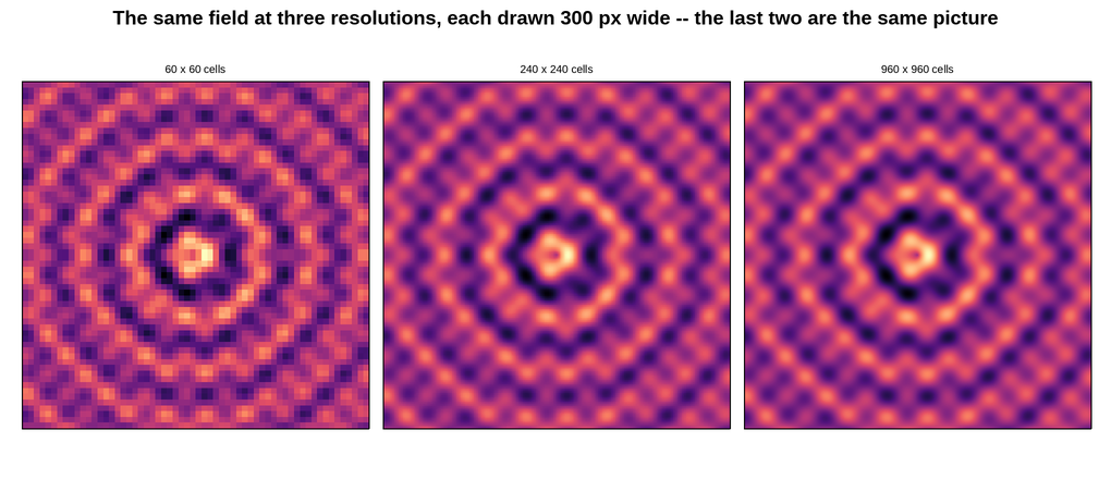
Past about one cell per output pixel, extra cells cannot appear. They are computed, normalised, colour-mapped and compressed, and then averaged away by the encoder or the display. The three panels are the same field at 60, 240 and 960 cells across, drawn at the same physical size: the first is visibly coarse, the second is at the display’s limit, and the third is indistinguishable from the second while costing 16 times the cells.

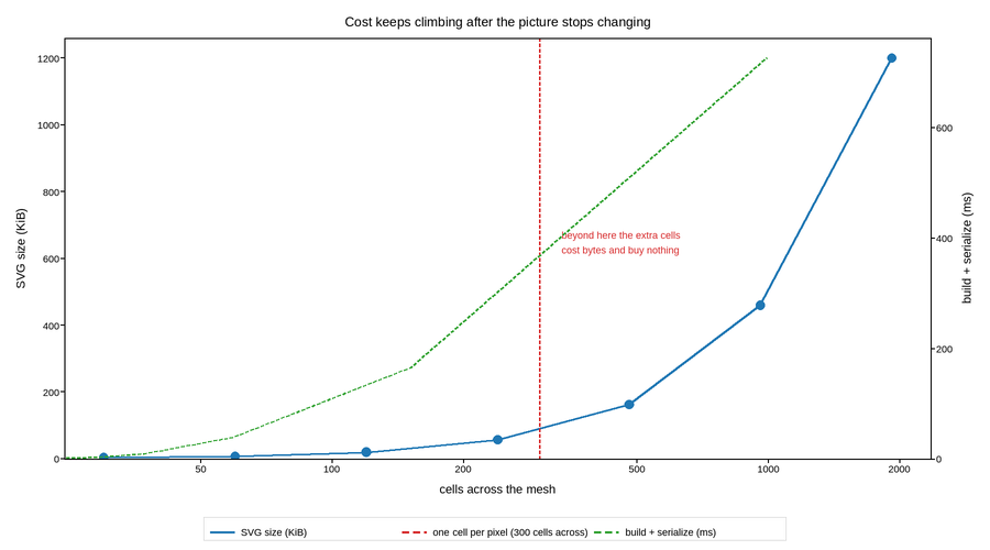
The lower panel measures the point at which that happens on this figure. To the left of the marked line, refining the grid buys visible detail; to the right it buys file size and build time only. This is worth knowing in the direction that usually bites – there is rarely a reason to hand pcolormesh a 4000-square array for a 500-pixel-wide axes – and it is the one place where downsampling your own data before plotting is strictly better than letting the library do it.

The other half of the trade is not measurable in a PNG: because the layer is an image, scaling the SVG up softens the field while the axes, ticks and any line artists over it stay sharp. For a field sampled far finer than the display that is the right trade. For a coarse mesh whose cell edges are the point, it is the wrong one – pcolormesh(..., rasterized=False) is the fallback there, forcing exact vector <rect> cells that stay crisp at any zoom (see Non-uniform meshes: vector cells by default, and when raster comes back). It is a fix for this problem specifically, sharp edges on a small, deliberately coarse grid, not for the one above: forcing it on any of the three panels here would still draw the same visibly-averaged 60/240/960-cell picture, just as one <rect> per cell instead of one <image> – vector geometry has no more cells to show than the array was given, only sharper edges on the ones it has.

• 
• 

Live figure — pick a tool, then zoom, pan, point-pick or annotate. Nothing is active until a tool is selected.

Live figure — pick a tool, then zoom, pan, point-pick or annotate. Nothing is active until a tool is selected.

import time

import numpy as np
import plotpress

RESOLUTIONS = [60, 240, 960]
PANEL_INCHES = 3.0                       # each panel is this wide, at dpi 100


def field(n):
    """A field with structure right down to the finest grid, so nothing here is
    redundant *in the data* -- only in what the display can show."""
    g = np.linspace(-3.0, 3.0, n)
    X, Y = np.meshgrid(g, g)
    R = np.hypot(X, Y)
    return g, np.sin(7.0 * R) / (1.0 + R) + 0.35 * np.sin(9.0 * X) * np.cos(9.0 * Y)


fig, axes = plotpress.subplots(1, len(RESOLUTIONS),
                               figsize=(PANEL_INCHES * len(RESOLUTIONS) + 1.2, 4.4))
for ax, n in zip(axes, RESOLUTIONS):
    g, Z = field(n)
    ax.pcolormesh(g, g, Z, cmap="magma")
    ax.set_aspect("equal")
    ax.set_xticks([])
    ax.set_yticks([])
    ax.set_title(f"{n} x {n} cells", size=10)

# Where the extra cells stop reaching the screen: the axes is this many pixels
# across, so a cell narrower than one of them cannot be resolved.
panel_px = PANEL_INCHES * fig.style.dpi
fig.suptitle(f"The same field at three resolutions, each drawn "
             f"{panel_px:.0f} px wide -- the last two are the same picture")
fig.tight_layout()

def cost_of(n):
    """(KiB, ms) for one mesh at this resolution.

    Inside a function so the scratch Figure stays local: the gallery scraper
    publishes every Figure left in an example's globals, and a measurement rig
    would appear as extra, meaningless images on the page.
    """
    g, Z = field(n)
    t0 = time.perf_counter()
    f, a = plotpress.subplots(figsize=(PANEL_INCHES, PANEL_INCHES))
    a.pcolormesh(g, g, Z, cmap="magma")
    kib = len(f.to_svg().encode("utf-8")) / 1024.0
    return kib, (time.perf_counter() - t0) * 1e3


sizes = [(n,) + cost_of(n) for n in (30, 60, 120, 240, 480, 960, 1920)]

cells = np.array([s[0] for s in sizes], dtype=float)
kib = np.array([s[1] for s in sizes])
ms = np.array([s[2] for s in sizes])

cost_fig, cost_ax = plotpress.subplots(figsize=(9.0, 5.0))
cost_ax.plot(cells, kib, color="#1f77b4", linewidth=2.0, label="SVG size (KiB)")
cost_ax.scatter(cells, kib, s=6.0, color="#1f77b4")
cost_ax.axvline(panel_px, color="#d62728", linestyle="--", linewidth=1.6,
                label=f"one cell per pixel ({panel_px:.0f} cells across)")
cost_ax.text(panel_px * 1.12, kib.max() * 0.55,
             "beyond here the extra cells\ncost bytes and buy nothing",
             fontsize=9, color="#d62728")

cost2 = cost_ax.twinx()
cost2.plot(cells, ms, color="#2ca02c", linewidth=1.6, linestyle="--",
           label="build + serialize (ms)")
cost2.set_ylabel("build + serialize (ms)")
cost2.set_ylim(0.0, None)

cost_ax.set_xscale("log")
cost_ax.set_xlabel("cells across the mesh")
cost_ax.set_ylabel("SVG size (KiB)")
cost_ax.set_ylim(0.0, None)
cost_ax.set_title("Cost keeps climbing after the picture stops changing")
cost_fig.legend(ax=[cost_ax, cost2], loc="lower center", ncol=3)
cost_fig.tight_layout()