Contour output is unbounded, and nothing caps it

contour is the one plot type in the library with no ceiling on its output. A mesh collapses to one image, a line decimates to the pixel column, a scatter batches into a single path – but contour lines are genuine vector geometry, and marching squares emits a segment per grid cell the level crosses. Nothing downstream thins them.

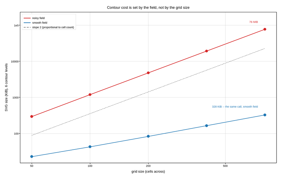
How bad that gets depends entirely on the field, not on its size, and this is the figure’s point. A smooth field has short, closed contours: their total length grows roughly with the grid’s linear dimension, so the file grows slowly and stays servable. A noisy field has contours that wander through nearly every cell, so their length grows with the grid’s area and the file grows with it.

The measured gap is several orders of magnitude at the same grid size. On this machine a 2000-square noisy field produces a few hundred megabytes of SVG – past what a browser will open, from a call that looks identical to the one that produces a hundred kilobytes.

There is no keyword to protect you, so the practical rules are: smooth the field before contouring it, keep the level count low, and if the field is genuinely noisy use pcolormesh or contourf, both of which rasterize and are therefore bounded. The dashed reference is slope 2 – proportional to the cell count – which the noisy series tracks and the smooth one does not.

Live figure — pick a tool, then zoom, pan, point-pick or annotate. Nothing is active until a tool is selected.

import numpy as np
import plotpress

rng = np.random.default_rng(0)

GRIDS = [50, 100, 200, 400, 800]
LEVELS = 6


def smooth_field(n):
    g = np.linspace(-3.0, 3.0, n)
    X, Y = np.meshgrid(g, g)
    return g, np.sin(X) * np.cos(Y) + 0.5 * np.exp(-(X ** 2 + Y ** 2) / 3.0)


def noisy_field(n):
    g = np.linspace(-3.0, 3.0, n)
    return g, rng.random((n, n))


def contour_kib(builder, n):
    g, Z = builder(n)
    f, a = plotpress.subplots(figsize=(5.0, 4.0))
    a.contour(g, g, Z, levels=LEVELS)
    return len(f.to_svg().encode("utf-8")) / 1024.0


smooth = [contour_kib(smooth_field, n) for n in GRIDS]
noisy = [contour_kib(noisy_field, n) for n in GRIDS]

grids = np.array(GRIDS, dtype=float)

fig, ax = plotpress.subplots(figsize=(9.2, 5.8))
ax.plot(grids, noisy, color="#d62728", linewidth=2.2, label="noisy field")
ax.scatter(grids, noisy, s=6.0, color="#d62728")
ax.plot(grids, smooth, color="#1f77b4", linewidth=2.2, label="smooth field")
ax.scatter(grids, smooth, s=6.0, color="#1f77b4")

# Slope 2 on log-log: output proportional to the cell count. Offset downward so
# it reads as a guide -- drawn through the data it would sit exactly under the
# noisy series, which is the finding but is invisible as two coincident lines.
ref = 0.30 * noisy[0] * (grids / grids[0]) ** 2
ax.plot(grids, ref, color="#888888", linestyle="--", linewidth=1.4,
        label="slope 2 (proportional to cell count)")

# Labelled at the line ends rather than with leaders: on a log axis a callout
# offset by a constant factor sits at almost the same height as its target, so
# the leader runs the width of the panel to travel no distance at all.
ax.text(grids[-1] * 0.92, noisy[-1] * 1.5, f"{noisy[-1] / 1024:.0f} MiB",
        color="#d62728", fontsize=9, ha="right")
ax.text(grids[-1] * 0.92, smooth[-1] * 1.6,
        f"{smooth[-1]:.0f} KiB -- the same call, smooth field",
        color="#1f77b4", fontsize=9, ha="right")

ax.set_xscale("log")
ax.set_yscale("log")
# Headroom for the label above the top line, which autoscaling does not leave.
ax.set_ylim(None, noisy[-1] * 3.0)
ax.set_xlabel("grid size (cells across)")
ax.set_ylabel(f"SVG size (KiB), {LEVELS} contour levels")
ax.set_title("Contour cost is set by the field, not by the grid size")
ax.legend(loc="upper left")
ax.grid(True)
fig.tight_layout()