Vector overlays on a rasterized field

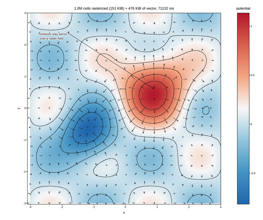
The mesh examples in this gallery make one trade – the field becomes an embedded image – and this is the figure that shows what it costs and what it does not.

A million-cell field is rasterized to a single <image>. Everything drawn over it stays vector: contour lines, a thinned quiver field, the annotation and its leader, the axes frame, the ticks. Zoom the SVG and the contours stay crisp while the field softens, which is the correct division of labour, because the contours are a computed boundary that means something at any magnification and the field is a sampling that does not.

That division is also why the contour count matters. Contours are the vector part, so they are the part whose node count scales: eight levels over a 1000-cell-square grid is a few thousand path segments, and forty levels would be five times that with no more information. The quiver is thinned for the same reason – one arrow per fifty cells – since a vector per cell would be twenty thousand arrows drawn on top of a field they are meant to annotate.

The figure reports the split, so the raster and vector halves of the file can be seen separately.

Live figure — pick a tool, then zoom, pan, point-pick or annotate. Nothing is active until a tool is selected.

import time

import numpy as np
import plotpress

N = 1000
g = np.linspace(-3.0, 3.0, N)
X, Y = np.meshgrid(g, g)

# A smooth potential and its gradient: the field is the raster layer, the
# contours and arrows are the vector ones.
Z = (np.exp(-((X - 0.9) ** 2 + (Y - 0.6) ** 2) / 1.1)
     - 0.8 * np.exp(-((X + 1.2) ** 2 + (Y + 0.8) ** 2) / 0.7)
     + 0.25 * np.sin(2.0 * X) * np.cos(2.0 * Y))
V, U = np.gradient(-Z, g, g)

t0 = time.perf_counter()
fig, ax = plotpress.subplots(figsize=(8.6, 7.2))
mesh = ax.pcolormesh(g, g, Z, cmap="RdBu_r")
bar = fig.colorbar(mesh, ax=ax)
bar.set_title("potential")

ax.contour(g, g, Z, levels=8, colors="#111111")

thin = slice(None, None, 50)                    # one arrow per 50x50 cells
ax.quiver(X[thin, thin], Y[thin, thin], U[thin, thin], V[thin, thin],
          color="#222222")

ax.annotate("contours stay vector\nover a raster field",
            xy=(0.9, 0.6), xytext=(-2.7, 2.3),
            arrowprops={"color": "#111111"}, fontsize=10)

ax.set_aspect("equal")
ax.set_xlabel("x")
ax.set_ylabel("y")
fig.tight_layout()
build_ms = (time.perf_counter() - t0) * 1e3

svg = fig.to_svg()
# The embedded images are the raster half; everything else is vector.
raster_kib = sum(len(chunk.split('"')[0]) for chunk in
                 svg.split("data:image/png;base64,")[1:]) / 1024.0
total_kib = len(svg.encode("utf-8")) / 1024.0
ax.set_title(f"{N * N / 1e6:.1f}M cells rasterized ({raster_kib:.0f} KiB) + "
             f"{total_kib - raster_kib:.0f} KiB of vector, {build_ms:.0f} ms")