A thousand series on one axes

The opposite stress from a million-point line: a thousand separate artists, each short. Here the per-series overhead is the whole cost – object construction, colour resolution, bounds computation, one path per series – and there is no decimation to hide behind, because every series must appear.

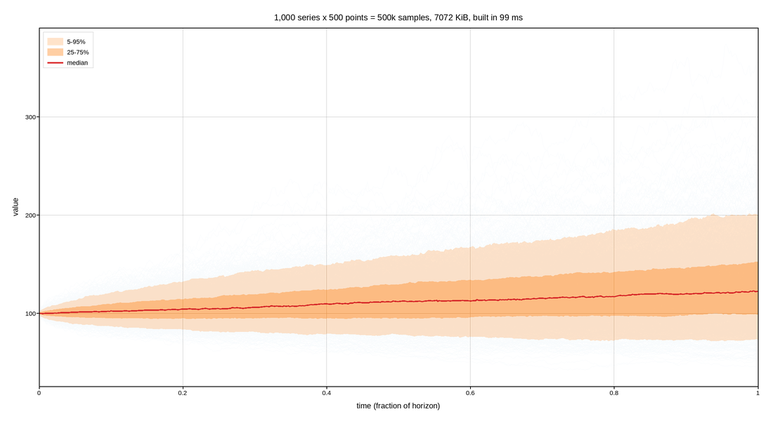
This is the shape a Monte Carlo fan chart takes, and it is drawn the way one should be: the individual paths at low opacity so their density reads as a distribution, with the quantile envelopes computed across the ensemble and drawn on top. The envelopes are what a reader actually measures; the paths are there to show that the envelope summarises something real and is not itself the model.

An ensemble of a thousand is also where the alpha has to be chosen against the count rather than by eye: at 1/1000 opacity per path the bundle reads as tone, and at the 0.4 that looks right for five series it would be a solid block.

Live figure — pick a tool, then zoom, pan, point-pick or annotate. Nothing is active until a tool is selected.

import time

import numpy as np
import plotpress

rng = np.random.default_rng(11)

N_PATHS = 1000
N_STEPS = 500
t = np.linspace(0.0, 1.0, N_STEPS)

# Geometric random walks with a common drift -- one row per path.
steps = rng.normal(0.0004, 0.014, (N_PATHS, N_STEPS))
paths = 100.0 * np.exp(np.cumsum(steps, axis=1))

quantiles = np.percentile(paths, [5, 25, 50, 75, 95], axis=0)

t0 = time.perf_counter()
fig, ax = plotpress.subplots(figsize=(11.0, 6.0))

# Opacity scaled to the ensemble size: the bundle should read as density.
for row in paths:
    ax.plot(t, row, color="#1f77b4", linewidth=0.4, alpha=0.03)

ax.fill_between(t, quantiles[0], quantiles[4], color="#ff7f0e", alpha=0.22,
                label="5-95%")
ax.fill_between(t, quantiles[1], quantiles[3], color="#ff7f0e", alpha=0.38,
                label="25-75%")
ax.plot(t, quantiles[2], color="#d62728", linewidth=2.2, label="median")

ax.set_xlim(0.0, 1.0)
ax.set_xlabel("time (fraction of horizon)")
ax.set_ylabel("value")
ax.legend(loc="upper left")
ax.grid(True)
fig.tight_layout()
build_ms = (time.perf_counter() - t0) * 1e3

svg = fig.to_svg()
ax.set_title(f"{N_PATHS:,} series x {N_STEPS} points = "
             f"{N_PATHS * N_STEPS / 1e3:.0f}k samples, "
             f"{len(svg) / 1024:.0f} KiB, built in {build_ms:.0f} ms")