Adaptive search for a halo, with the adaptive package

Every other sparse-sampling example in this gallery picks its sample positions before the run starts (random, raster, growing bounds) or implicitly (wherever a sensor happened to be installed). adaptive picks them during the run: after each batch of evaluations, its Learner2D looks at where the function is varying fastest and asks for the next points there, rather than spending its evaluation budget uniformly over a domain that’s mostly flat. That’s a genuinely different search strategy from Both axes growing: a search window expanding outward’s expanding window: the domain here is fixed and known from the start (a real sweep range), but where within it is worth measuring isn’t.

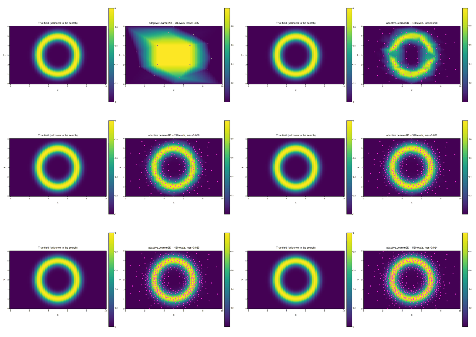
The target here is a ring, not a simple Gaussian blob – deliberately, so the payoff of adaptive sampling is more obvious than it would be on a single peak. A ring has two steep edges (inner and outer) wrapped around a flat, uninteresting center, so a strategy that greedily concentrates on “whichever single point looks steepest” would get stuck resolving one arc of it – the learner instead has to keep spreading its budget around the whole ring as it comes into focus, which is exactly what its scatter shows happening frame to frame.

The right panel’s scatter is exactly what the learner has chosen to evaluate so far, and its background is Learner2D.interpolated_on_grid() – the package’s own reconstruction from those points, not a hand-rolled interpolator, on the same fixed grid every frame so only the sample placement changes frame to frame.

The code below is exactly what you’d write against the real plotpress.qt.LiveArtist: a callback that receives the search’s newest batch of measurements and redraws, fed by a loop that asks the learner where to measure next, “measures” it, and reports back. Only measure() is meant to be replaced, with your own instrument call – the adaptive.Learner2D driving where to measure doesn’t change at all, live or not.

import adaptive
import numpy as np
import plotpress


BOUNDS = [(0.0, 10.0), (0.0, 6.0)]
GRID_N = 60          # background resolution -- fixed, so only the
                      # scatter's placement (not the grid) changes


def true_field(x, y):
    # Only used to draw the left, "ground truth" reference panel -- the
    # search itself never sees this, only what measure() reports back.
    r = np.hypot(x - RING_CENTER[0], y - RING_CENTER[1])
    return np.exp(-((r - RING_RADIUS) ** 2) / (2.0 * RING_SIGMA ** 2))


RING_CENTER = (5.0, 3.0)
RING_RADIUS = 2.0
RING_SIGMA = 0.35
tx = np.linspace(BOUNDS[0][0], BOUNDS[0][1], GRID_N)
ty = np.linspace(BOUNDS[1][0], BOUNDS[1][1], GRID_N)
TX, TY = np.meshgrid(tx, ty)
truth_grid = true_field(TX, TY)

fig, (ax_true, ax_recon) = plotpress.subplots(1, 2, figsize=(11, 5.2))

m_true = ax_true.pcolormesh(tx, ty, truth_grid, cmap="viridis", vmin=0, vmax=1)
ax_true.set_aspect("equal")
ax_true.set_title("True field (unknown to the search)")
ax_true.set_xlabel("x"); ax_true.set_ylabel("y")
fig.colorbar(m_true, ax=ax_true)

recon_mesh = LiveArtist(ax_recon, cmap="viridis")   # no vmin/vmax -- autoscales
_cbar_ax = None


def on_new_batch(xs, ys, recon_grid, sample_xy, npoints, loss):
    """Called once per acquisition tick with the search's current
    reconstruction and its own progress diagnostics.
    """
    global _cbar_ax
    recon_mesh.update(xs, ys, recon_grid)
    # Magenta barely appears anywhere in viridis' own range, so a marker
    # small enough to still show most of the cell color underneath it
    # stays readable at every point along the ring, not just where it
    # happens to land on a light or dark patch of the colormap.
    ax_recon.scatter(sample_xy[:, 0], sample_xy[:, 1], color="#ff2fd4", s=3)
    ax_recon.set_aspect("equal")             # cla() inside update() wiped these
    ax_recon.set_xlim(*BOUNDS[0]); ax_recon.set_ylim(*BOUNDS[1])
    ax_recon.set_title(f"adaptive.Learner2D -- {npoints} evals, loss={loss:.3f}")
    ax_recon.set_xlabel("x"); ax_recon.set_ylabel("y")
    # Autoscaled, unlike the true field's fixed 0-1 scale: early on, with
    # only a handful of points, the interpolation hasn't found the ring's
    # real height yet, so its own range is a running readout of how much
    # of it the search has actually resolved so far.
    if _cbar_ax is not None:
        fig.delaxes(_cbar_ax)
    _cbar_ax = fig.colorbar(recon_mesh.last_artist, ax=ax_recon)
    fig.tight_layout()


# ---------------------------------------------------------------------------
# Data acquisition -- replace this with your own instrument. Everything
# above only needs a reconstructed grid and the search's own diagnostics
# handed to on_new_batch() as each batch of measurements completes. The
# adaptive.Learner2D driving *where* to measure doesn't change at all.
# ---------------------------------------------------------------------------
POINTS_PER_TICK = 20
N_TICKS = 26


def measure(xy):
    """Stand-in for the instrument reporting a reading at (x, y)."""
    x, y = xy
    return float(true_field(x, y))


learner = adaptive.Learner2D(measure, bounds=BOUNDS)


def read_next_batch():
    """Ask the search where to measure next, measure those points, and
    return its current reconstruction.
    """
    new_points, _ = learner.ask(POINTS_PER_TICK)
    for p in new_points:
        learner.tell(p, measure(p))
    xs, ys, zs = learner.interpolated_on_grid(n=GRID_N)
    recon_grid = zs.T   # interpolated_on_grid is (x, y) indexed; pcolormesh wants (y, x)
    sample_xy = np.array(list(learner.data.keys()))
    return xs, ys, recon_grid, sample_xy, learner.npoints, learner.loss()


for _ in range(N_TICKS):
    on_new_batch(*read_next_batch())