Cyclic voltammetry, cycle over cycle

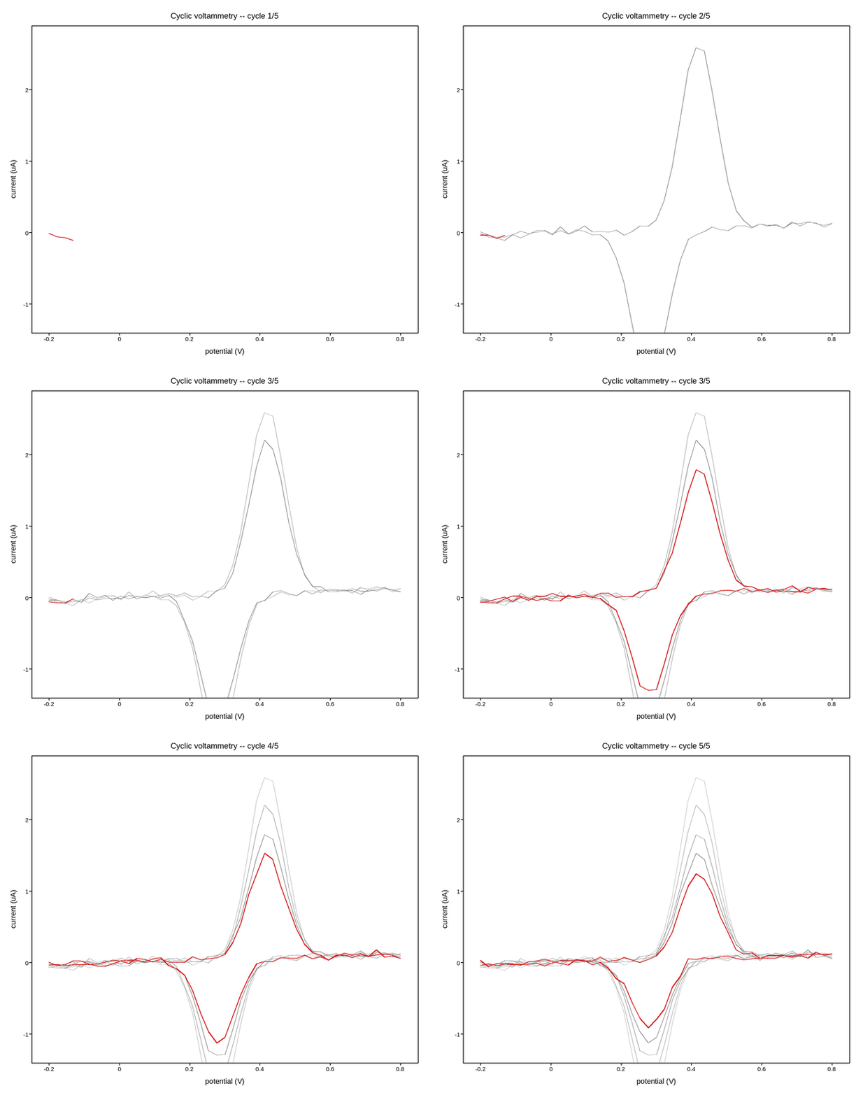
A cyclic voltammogram sweeps voltage forward then back across a fixed window, tracing out a loop – both axes are bounded and known before the run starts, unlike every growing-axis example elsewhere in this gallery. What makes it worth its own example is what happens between cycles: each new sweep retraces the same loop, drawn over the earlier ones rather than replacing them, so cycle-to-cycle drift (here, a fouling electrode losing peak current) shows up directly as the loops shrink inward over the run.

Structured the way a real acquisition script would be: a callback that receives the next chunk of the current cycle’s trace and redraws, fed here by a loop simulating the potentiostat. This needs the current cycle drawn on top of the faded, semi-transparent older ones, and plotpress.qt.LiveArtist – like plain ax.cla() – clears the whole axes on every update(), so there’s no way to layer a fresh call over what a previous one drew; the honest turn-key version manages the whole redraw directly (ax.cla(), older cycles first, current cycle last) the same way this does, rather than force it through an artist wrapper built for one series at a time.

import numpy as np
import plotpress


V_MIN, V_MAX = -0.2, 0.8   # the sweep window, fixed by the method

fig, ax = plotpress.subplots(figsize=(6.5, 5.5))
completed_cycles = []   # each: (voltage_full, current_full)
current_v, current_i = [], []


def on_new_samples(v_chunk, i_chunk):
    """Called once per acquisition tick with the next chunk of the current
    cycle's (voltage, current) trace.
    """
    current_v.extend(v_chunk)
    current_i.extend(i_chunk)

    ax.cla()
    for j, (v_old, i_old) in enumerate(completed_cycles):
        fade = 0.15 + 0.5 * (j + 1) / max(1, len(completed_cycles))
        ax.plot(v_old, i_old, color="#555555", alpha=fade, linewidth=1.0)
    ax.plot(current_v, current_i, color="#d62728", linewidth=1.6)
    ax.set_xlim(V_MIN - 0.05, V_MAX + 0.05)
    ax.set_ylim(-1.4, 2.9)
    ax.set_xlabel("potential (V)"); ax.set_ylabel("current (uA)")
    ax.set_title(f"Cyclic voltammetry -- cycle {len(completed_cycles) + 1}/{N_CYCLES}")
    fig.tight_layout()


def on_cycle_complete():
    """Called when a full forward+reverse sweep finishes -- archive it as
    one of the faded background traces and start the next cycle fresh.
    """
    global current_v, current_i
    completed_cycles.append((current_v, current_i))
    current_v, current_i = [], []


# ---------------------------------------------------------------------------
# Data acquisition -- replace this with your own potentiostat driver. Every-
# thing above only needs a chunk of (voltage, current) handed to
# on_new_samples() as it's measured, and on_cycle_complete() called once
# each sweep finishes.
# ---------------------------------------------------------------------------
rng = np.random.default_rng(14)
POINTS_PER_HALF = 45
N_CYCLES = 5
STRIDE = 4

forward = np.linspace(V_MIN, V_MAX, POINTS_PER_HALF)
reverse = np.linspace(V_MAX, V_MIN, POINTS_PER_HALF)[1:]
voltage_cycle = np.concatenate([forward, reverse])


def read_next_chunk(cycle_index, lo, hi):
    """Stand-in for the potentiostat reporting its newest samples --
    redox peaks (oxidation on the forward sweep, reduction on the reverse)
    that shrink each cycle as the electrode fouls, plus a capacitive
    background and measurement noise.
    """
    v = voltage_cycle[lo:hi]
    is_forward = np.arange(lo, hi) < POINTS_PER_HALF
    decay = 0.82 ** cycle_index
    i = 0.15 * v
    i = i + np.where(is_forward, 1.0, 0.0) * decay * 2.6 * np.exp(-((v - 0.42) ** 2) / (2 * 0.05 ** 2))
    i = i - np.where(is_forward, 0.0, 1.0) * decay * 2.1 * np.exp(-((v - 0.28) ** 2) / (2 * 0.05 ** 2))
    return v, i + 0.03 * rng.standard_normal(v.shape)


for cycle_index in range(N_CYCLES):
    for lo in range(0, len(voltage_cycle), STRIDE):
        hi = min(lo + STRIDE, len(voltage_cycle))
        on_new_samples(*read_next_chunk(cycle_index, lo, hi))
    on_cycle_complete()