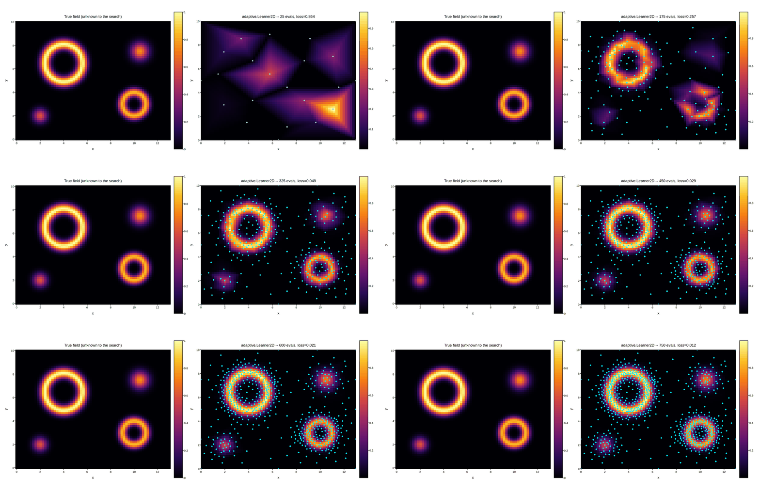
Adaptive search across several separated anomalies

Adaptive search for a halo, with the adaptive package has exactly one feature to find. A real sweep – a defect scan, a multi-resonance spectroscopy map – more often has several, scattered across a domain that’s mostly featureless in between, and not all of the same shape. Four unrelated structures sit here: two rings of different size and two compact point anomalies, none overlapping. adaptive.Learner2D has no idea any of this exists going in – it starts from the four corners and center, the same as Adaptive search for a halo, with the adaptive package does, and has to discover all four regions on its own budget, not just the first one it stumbles onto, while still not wasting samples on the large flat gaps between them.

The code below is exactly what you’d write against the real plotpress.qt.LiveArtist: a callback that receives the search’s newest batch of measurements and redraws, fed by a loop that asks the learner where to measure next, “measures” it, and reports back. Only measure() is meant to be replaced, with your own instrument call – the adaptive.Learner2D driving where to measure doesn’t change at all, live or not.

import adaptive
import numpy as np
import plotpress


BOUNDS = [(0.0, 13.0), (0.0, 10.0)]
GRID_N = 65          # background resolution -- fixed, so only the
                      # scatter's placement (not the grid) changes

# (kind, center, ring radius (None for a blob), sigma, peak amplitude)
STRUCTURES = [
    ("ring", (4.0, 6.5), 1.6, 0.30, 1.0),
    ("ring", (10.0, 3.0), 1.0, 0.25, 0.85),
    ("blob", (10.5, 7.5), None, 0.50, 0.75),
    ("blob", (2.0, 2.0), None, 0.40, 0.60),
]


def true_field(x, y):
    # Only used to draw the left, "ground truth" reference panel -- the
    # search itself never sees this, only what measure() reports back.
    total = 0.0
    for kind, (cx, cy), size, sigma, amp in STRUCTURES:
        r = np.hypot(x - cx, y - cy)
        bump = amp * np.exp(-(r ** 2) / (2.0 * sigma ** 2)) if kind == "blob" else \
               amp * np.exp(-((r - size) ** 2) / (2.0 * sigma ** 2))
        total = np.maximum(total, bump)
    return total


tx = np.linspace(BOUNDS[0][0], BOUNDS[0][1], GRID_N)
ty = np.linspace(BOUNDS[1][0], BOUNDS[1][1], GRID_N)
TX, TY = np.meshgrid(tx, ty)
truth_grid = true_field(TX, TY)

fig, (ax_true, ax_recon) = plotpress.subplots(1, 2, figsize=(12, 5.2))

m_true = ax_true.pcolormesh(tx, ty, truth_grid, cmap="inferno", vmin=0, vmax=1)
ax_true.set_aspect("equal")
ax_true.set_title("True field (unknown to the search)")
ax_true.set_xlabel("x"); ax_true.set_ylabel("y")
fig.colorbar(m_true, ax=ax_true)

recon_mesh = LiveArtist(ax_recon, cmap="inferno")   # no vmin/vmax -- autoscales
_cbar_ax = None


def on_new_batch(xs, ys, recon_grid, sample_xy, npoints, loss):
    """Called once per acquisition tick with the search's current
    reconstruction and its own progress diagnostics.
    """
    global _cbar_ax
    recon_mesh.update(xs, ys, recon_grid)
    # Cyan is a hue inferno's own black-purple-red-orange-yellow range never
    # touches, so a small marker stays visible over every part of it without
    # covering much of the cell color it's sitting on.
    ax_recon.scatter(sample_xy[:, 0], sample_xy[:, 1], color="#00e5ff", s=3)
    ax_recon.set_aspect("equal")             # cla() inside update() wiped these
    ax_recon.set_xlim(*BOUNDS[0]); ax_recon.set_ylim(*BOUNDS[1])
    ax_recon.set_title(f"adaptive.Learner2D -- {npoints} evals, loss={loss:.3f}")
    ax_recon.set_xlabel("x"); ax_recon.set_ylabel("y")
    # Autoscaled, unlike the true field's fixed 0-1 scale: until every
    # structure has been found, the reconstruction's own range is a running
    # readout of how much of the strongest one so far has been resolved.
    if _cbar_ax is not None:
        fig.delaxes(_cbar_ax)
    _cbar_ax = fig.colorbar(recon_mesh.last_artist, ax=ax_recon)
    fig.tight_layout()


# ---------------------------------------------------------------------------
# Data acquisition -- replace this with your own instrument. Everything
# above only needs a reconstructed grid and the search's own diagnostics
# handed to on_new_batch() as each batch of measurements completes. The
# adaptive.Learner2D driving *where* to measure doesn't change at all.
# ---------------------------------------------------------------------------
POINTS_PER_TICK = 25
N_TICKS = 30


def measure(xy):
    """Stand-in for the instrument reporting a reading at (x, y)."""
    x, y = xy
    return float(true_field(x, y))


learner = adaptive.Learner2D(measure, bounds=BOUNDS)


def read_next_batch():
    """Ask the search where to measure next, measure those points, and
    return its current reconstruction.
    """
    new_points, _ = learner.ask(POINTS_PER_TICK)
    for p in new_points:
        learner.tell(p, measure(p))
    xs, ys, zs = learner.interpolated_on_grid(n=GRID_N)
    recon_grid = zs.T   # interpolated_on_grid is (x, y) indexed; pcolormesh wants (y, x)
    sample_xy = np.array(list(learner.data.keys()))
    return xs, ys, recon_grid, sample_xy, learner.npoints, learner.loss()


for _ in range(N_TICKS):
    on_new_batch(*read_next_batch())