Hertzsprung-Russell diagram of a star cluster

The single most conventional plot in astronomy, and one whose conventions are all backwards. Colour index runs blue to red, which means hot to cool, which means the temperature axis increases to the left. Absolute magnitude is a logarithmic brightness scale that runs backwards too – smaller numbers are brighter – so the y axis is inverted as well. Both are done with invert_xaxis / invert_yaxis rather than by negating the data, so the tick labels still read as the catalogue quotes them.

The astrophysics is in the shape. Stars spend most of their lives on the main sequence, the diagonal band; when they exhaust core hydrogen they leave it and climb to the giant branch. The magnitude at which the cluster’s main sequence ends is the cluster’s age, which is why the turn-off point is worth annotating rather than leaving to the reader to find.

Roughly ten thousand stars would be an unreadable blot as opaque markers, so they are drawn small and semi-transparent: the density of the main sequence then shows through as tone, and the sparse giant branch stays visible instead of being drowned.

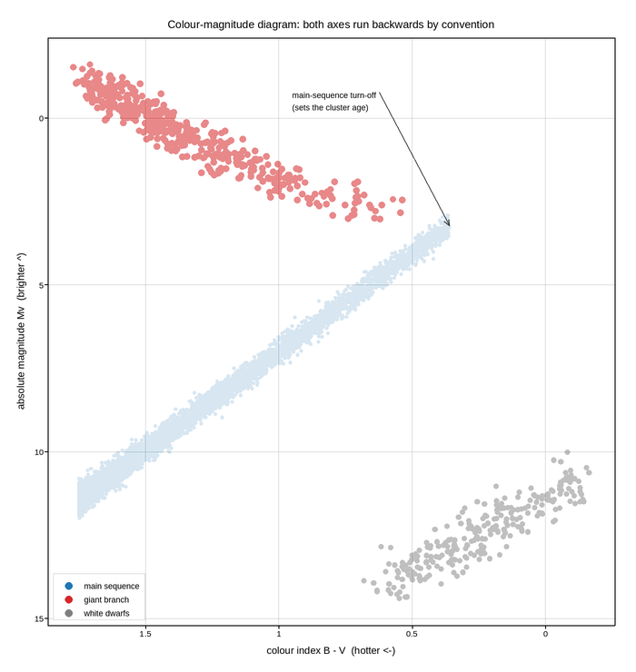
Live figure — pick a tool, then zoom, pan, point-pick or annotate. Nothing is active until a tool is selected.

View this figure’s Vega export ↗ — the raw JSON spec, rendered live by a real Vega engine.

View this figure’s Vega-Lite export ↗ — the raw JSON spec(s), rendered live by a real Vega-Lite engine.

import numpy as np
import polars as pl
import plotpress

rng = np.random.default_rng(5150)

N_MAIN = 9000
N_GIANT = 420
N_WD = 260

# Main sequence: a mass function that produces far more faint red stars than
# bright blue ones, mapped onto a colour-magnitude relation.
u = rng.power(0.35, N_MAIN)                       # skewed toward faint stars
bv_main = 1.75 - 1.95 * u
mv_main = 5.9 * bv_main + 1.1 + rng.normal(0.0, 0.18, N_MAIN)

TURNOFF_BV = 0.36                                 # cluster age shows up here
above = bv_main < TURNOFF_BV
bv_main, mv_main = bv_main[~above], mv_main[~above]

# Giant branch: leaves the main sequence at the turn-off and climbs. Stars
# evolve up it quickly, so it is sparsely populated -- weighting toward the base
# is what keeps it a branch rather than a second solid band.
s = rng.power(2.0, N_GIANT)
bv_giant = TURNOFF_BV + 1.35 * s ** 0.8 + rng.normal(0.0, 0.05, N_GIANT)
mv_giant = (3.0 - 4.2 * s ** 1.4) + rng.normal(0.0, 0.25, N_GIANT)

# White dwarfs: hot, faint, and cooling along a track down and to the right --
# not a uniform box, which is what a naive rng.uniform pair would draw.
u = rng.random(N_WD)
bv_wd = -0.15 + 0.75 * u + rng.normal(0.0, 0.05, N_WD)
mv_wd = 10.8 + 3.2 * u + rng.normal(0.0, 0.35, N_WD)

# One row per catalogued star, one table per population -- the shape a
# photometric survey's own star catalogue is in, before it is split by
# evolutionary stage for the colour-magnitude diagram.
main_seq = pl.DataFrame({"bv": bv_main, "mv": mv_main})
giants = pl.DataFrame({"bv": bv_giant, "mv": mv_giant})
white_dwarfs = pl.DataFrame({"bv": bv_wd, "mv": mv_wd})
bv_main, mv_main = main_seq["bv"].to_numpy(), main_seq["mv"].to_numpy()
bv_giant, mv_giant = giants["bv"].to_numpy(), giants["mv"].to_numpy()
bv_wd, mv_wd = white_dwarfs["bv"].to_numpy(), white_dwarfs["mv"].to_numpy()

fig, ax = plotpress.subplots(figsize=(7.0, 7.4))
ax.scatter(bv_main, mv_main, s=2.6, color="#1f77b4", alpha=0.18,
           label="main sequence")
ax.scatter(bv_giant, mv_giant, s=5.0, color="#d62728", alpha=0.55,
           label="giant branch")
ax.scatter(bv_wd, mv_wd, s=4.0, color="#7f7f7f", alpha=0.5,
           label="white dwarfs")

ax.annotate("main-sequence turn-off\n(sets the cluster age)",
            xy=(TURNOFF_BV, 5.9 * TURNOFF_BV + 1.1),
            xytext=(0.95, -0.6), arrowprops={"color": "#333333"}, fontsize=9)

ax.invert_xaxis()                                 # hot stars on the left
ax.invert_yaxis()                                 # bright stars at the top
ax.set_xlabel("colour index B - V  (hotter <-)")
ax.set_ylabel("absolute magnitude Mv  (brighter ^)")
ax.set_title("Colour-magnitude diagram: both axes run backwards by convention")
ax.legend(loc="lower left")
ax.grid(True)
fig.tight_layout()