Exoplanet transit light curve

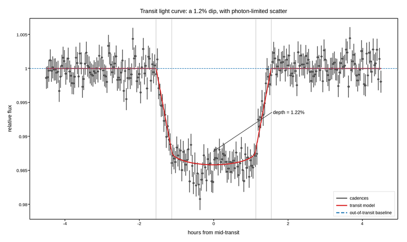
A planet crossing its star drops the measured flux by the area ratio of the two discs – here about 1.2%, which is a large transit and still a change of one part in eighty. Everything about the figure is arranged so that a change that small is legible.

Flux is plotted normalised to the out-of-transit baseline, so the y axis reads as fractional depth and the quantity being measured is the number the eye lands on. The axis is deliberately not zero-based: including zero would squash the entire transit into the top 1% of the panel. That is normally a warning sign, but here the baseline is a measured reference rather than an arbitrary crop, and it is drawn explicitly.

The individual cadences are scattered with their photometric errors, and the transit model is drawn over them. The point of the error bars is that they are comparable to the scatter – that is what tells you the noise is photon-limited and the detection is real, rather than the model being drawn through a cloud of systematics. The contact points are marked, because ingress duration is what constrains the impact parameter.

Live figure — pick a tool, then zoom, pan, point-pick or annotate. Nothing is active until a tool is selected.

View this figure’s Vega export ↗ — the raw JSON spec, rendered live by a real Vega engine.

View this figure’s Vega-Lite export ↗ — the raw JSON spec(s), rendered live by a real Vega-Lite engine.

import numpy as np
import polars as pl
import plotpress

rng = np.random.default_rng(314)

DEPTH = 0.0122                                    # (Rp/Rs)^2
T_TOTAL = 3.1                                     # first to fourth contact (hours)
T_INGRESS = 0.42                                  # contact 1 to contact 2 (hours)
SIGMA = 0.0016                                    # per-cadence photometric noise

t = np.linspace(-4.5, 4.5, 260)                   # hours from mid-transit

half_total = T_TOTAL / 2.0
half_flat = half_total - T_INGRESS


def transit_profile(t):
    """Trapezoidal transit with limb-darkened curvature across the floor."""
    a = np.abs(t)
    frac = np.clip((half_total - a) / T_INGRESS, 0.0, 1.0)
    # Limb darkening deepens the floor toward mid-transit.
    limb = 1.0 + 0.16 * np.sqrt(np.clip(1.0 - (a / half_flat) ** 2, 0.0, 1.0))
    return 1.0 - DEPTH * frac * np.where(a < half_flat, limb, 1.0)


model = transit_profile(t)
flux = model + rng.normal(0.0, SIGMA, t.size)
# A slow instrumental trend, the sort a detrending step is meant to remove.
flux += 4.0e-4 * np.sin(t / 3.4)

# One row per cadence -- the shape a photometry pipeline's own light-curve
# export is in, before the transit model is drawn over it.
cadences = pl.DataFrame({"t": t, "flux": flux})
t = cadences["t"].to_numpy()
flux = cadences["flux"].to_numpy()

fine = np.linspace(-4.5, 4.5, 1200)

fig, ax = plotpress.subplots(figsize=(8.4, 5.0))
ax.errorbar(t, flux, yerr=SIGMA, color="#555555", marker="o", markersize=3.0,
            linestyle="none", capsize=0.0, alpha=0.75, label="cadences")
ax.plot(fine, transit_profile(fine), color="#d62728", linewidth=1.8,
        label="transit model")
ax.axhline(1.0, color="#1f77b4", linestyle="--", linewidth=1.0,
           label="out-of-transit baseline")

for contact, style in [(-half_total, ":"), (-half_flat, ":"),
                       (half_flat, ":"), (half_total, ":")]:
    ax.axvline(contact, color="#999999", linestyle=style, linewidth=0.9)

ax.annotate(f"depth = {DEPTH * 1e2:.2f}%", xy=(0.0, 1.0 - DEPTH),
            xytext=(1.6, 1.0 - 0.55 * DEPTH), arrowprops={"color": "#333333"},
            fontsize=10)
ax.set_xlabel("hours from mid-transit")
ax.set_ylabel("relative flux")
ax.set_title("Transit light curve: a 1.2% dip, with photon-limited scatter")
ax.legend(loc="lower right")
fig.tight_layout()