BER bathtub curve and extrapolated jitter budget

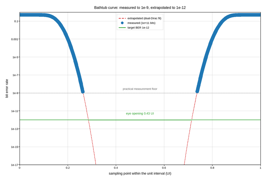
Bit error rate against where in the unit interval the receiver samples. The curve is called a bathtub for its shape: errors are certain near either data edge, fall away steeply as the sampling point moves into the eye, and reach a floor in the middle.

The y axis has to be logarithmic, and over more decades than any other plot in this gallery. A link specified at 1e-12 errors per bit is one error every hundred seconds at 10 Gb/s, so the interesting part of the curve is twelve decades below the part that is quick to measure. Ten decades of a linear axis is not a compromise; it is a blank sheet with a spike at each end.

That also settles how the figure is built. Errors below about 1e-9 cannot be counted in a reasonable test time, so measurement stops there and the rest is extrapolated – the tails of a bathtub are Gaussian, which is a straight line on a log-error axis against a normal quantile. The measured region is therefore drawn as points and the extrapolation as a dashed line, with the changeover marked. Presenting an extrapolation as though it were data is the standard way this plot gets misused; drawing them differently is the fix.

The eye opening quoted at the target BER is the horizontal distance between the two extrapolated walls, which is the number the link budget is spent from.

Live figure — pick a tool, then zoom, pan, point-pick or annotate. Nothing is active until a tool is selected.

View this figure’s Vega export ↗ — the raw JSON spec, rendered live by a real Vega engine.

View this figure’s Vega-Lite export ↗ — the raw JSON spec(s), rendered live by a real Vega-Lite engine.

import numpy as np
import polars as pl
import plotpress

rng = np.random.default_rng(555)

TARGET_BER = 1e-12
MEASURABLE = 1e-9                                  # floor of a practical test
RJ = 0.021                                         # random jitter, UI rms
DJ = 0.28                                          # deterministic jitter, UI pk-pk


def gaussian_tail(z):
    """Q(z) via an accurate erfc approximation -- no SciPy dependency."""
    t = 1.0 / (1.0 + 0.2316419 * np.abs(z))
    poly = t * (0.319381530 + t * (-0.356563782 + t * (1.781477937
                + t * (-1.821255978 + t * 1.330274429))))
    tail = 0.3989422804014327 * np.exp(-0.5 * z ** 2) * poly
    return np.where(z >= 0, tail, 1.0 - tail)


ui = np.linspace(0.0, 1.0, 801)
# Two Gaussian walls, one from each edge, separated by the deterministic jitter.
left_edge, right_edge = DJ / 2.0, 1.0 - DJ / 2.0
ber = 0.5 * (gaussian_tail((ui - left_edge) / RJ)
             + gaussian_tail((right_edge - ui) / RJ))
ber = np.clip(ber, 1e-18, 0.5)

# One row per sampling phase -- the shape a dual-Dirac fit's own model curve
# is in, before the measurable region is split out and given test noise.
model = pl.DataFrame({"ui": ui, "ber": ber})
ui = model["ui"].to_numpy()
ber = model["ber"].to_numpy()

measured = ber >= MEASURABLE
# Counting statistics: a measured BER of p over N bits has relative error
# 1/sqrt(N p), which is why the low end of the measured range is the noisy end.
N_BITS = 1e11
rel = 1.0 / np.sqrt(N_BITS * ber[measured])
ber_meas = ber[measured] * np.exp(rng.normal(0.0, np.minimum(rel, 0.6)))

# Eye opening at the target: where each extrapolated wall crosses TARGET_BER.
z_target = 6.9                                     # Q for 1e-12, two-sided
opening = (right_edge - z_target * RJ) - (left_edge + z_target * RJ)

fig, ax = plotpress.subplots(figsize=(8.6, 5.8))
ax.plot(ui, ber, color="#d62728", linestyle="--", linewidth=1.6,
        label="extrapolated (dual-Dirac fit)")
ax.scatter(ui[measured], ber_meas, s=8.0, color="#1f77b4",
           label=f"measured ({N_BITS:.0e} bits)")

ax.axhline(MEASURABLE, color="#888888", linestyle=":", linewidth=1.2)
ax.text(0.5, MEASURABLE * 2.2, "practical measurement floor", ha="center",
        fontsize=9, color="#666666")
ax.axhline(TARGET_BER, color="#2ca02c", linestyle="-", linewidth=1.4,
           label=f"target BER {TARGET_BER:.0e}")

ax.plot([left_edge + z_target * RJ, right_edge - z_target * RJ],
        [TARGET_BER, TARGET_BER], color="#2ca02c", linewidth=4.0, alpha=0.5)
ax.text(0.5, TARGET_BER * 4.0, f"eye opening {opening:.2f} UI", ha="center",
        fontsize=10, color="#2ca02c")

ax.set_yscale("log")
ax.set_ylim(1e-17, 1.0)
ax.set_xlim(0.0, 1.0)
ax.set_xlabel("sampling point within the unit interval (UI)")
ax.set_ylabel("bit error rate")
ax.set_title("Bathtub curve: measured to 1e-9, extrapolated to 1e-12")
ax.legend(loc="upper center")
ax.grid(True)
fig.tight_layout()