Photoluminescence in a magnetic field (LogNorm)

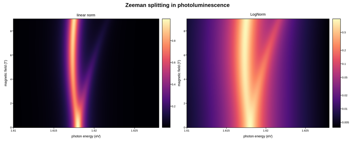
PL spectra of an excitonic emitter swept over magnetic field, showing Zeeman splitting of the emission line into two circularly polarized branches that separate linearly in B, on top of a quadratic diamagnetic shift.

E_pm(B) = E0 + sigma B^2 +/- g mu_B B / 2

The lower branch brightens with field while the upper one dims, because the two states thermalize – the Boltzmann factor across a splitting comparable to kT is what makes the map asymmetric rather than a simple fork.

PL intensity is the reason for the color scale. Emission at the line center is three to four orders of magnitude above the tails, so a linear norm shows two thin bright curves against black and discards the lineshape entirely. LogNorm puts each decade on equal footing and makes the weak wings and the background legible at the same time. The data is strictly positive, which is what makes a log scale admissible at all – a floor is added for the detector background so no cell is zero.

Live figure — pick a tool, then zoom, pan, point-pick or annotate. Nothing is active until a tool is selected.

View this figure’s Vega export ↗ — the raw JSON spec, rendered live by a real Vega engine.

View this figure’s Vega-Lite export ↗ — the raw JSON spec(s), rendered live by a real Vega-Lite engine.

import numpy as np
import polars as pl
import plotpress

E0 = 1.6180              # zero-field emission energy (eV)
G_FACTOR = 8.0           # exciton g factor
MU_B = 5.788e-5          # Bohr magneton (eV / T)
DIAMAGNETIC = 2.0e-5     # eV / T^2
LINEWIDTH = 0.0006       # half-width (eV)
KT = 0.0015              # ~17 K in eV
BACKGROUND = 3.0e-4      # detector floor, keeps every cell positive

energy = np.linspace(1.610, 1.628, 380)       # eV
field = np.linspace(0.0, 9.0, 300)            # T
E, B = np.meshgrid(energy, field)

center = E0 + DIAMAGNETIC * B ** 2
splitting = G_FACTOR * MU_B * B
lower = center - splitting / 2.0
upper = center + splitting / 2.0

# Thermal occupation: the upper branch depopulates once the splitting exceeds kT.
weight_upper = np.exp(-splitting / KT)
norm = 1.0 + weight_upper


def lorentzian(detuning, width):
    return width ** 2 / (detuning ** 2 + width ** 2)


intensity = (lorentzian(E - lower, LINEWIDTH) / norm
             + weight_upper * lorentzian(E - upper, LINEWIDTH) / norm)
intensity += BACKGROUND

# One row per (field, energy) spectrometer bin -- the shape a field-swept PL
# scan is actually recorded in, before it is gridded for the mesh.
sweep = pl.DataFrame({"energy": E.ravel(), "field": B.ravel(), "intensity": intensity.ravel()}) \
    .sort(["field", "energy"])
energy = sweep["energy"].unique().sort().to_numpy()
field = sweep["field"].unique().sort().to_numpy()
intensity = sweep["intensity"].to_numpy().reshape(field.size, energy.size)

fig, axes = plotpress.subplots(1, 2, figsize=(11.5, 4.6))
linear = axes[0].pcolormesh(energy, field, intensity, cmap="magma")
axes[0].set_title("linear norm")
fig.colorbar(linear, ax=axes[0])

log = axes[1].pcolormesh(energy, field, intensity, cmap="magma",
                         norm=plotpress.LogNorm())
axes[1].set_title("LogNorm")
fig.colorbar(log, ax=axes[1])

for ax in axes:
    ax.set_xlabel("photon energy (eV)")
    ax.set_ylabel("magnetic field (T)")
fig.suptitle("Zeeman splitting in photoluminescence")
fig.tight_layout()