Anharmonicity from flux-swept 0-1 and two-photon 0-2 spectroscopy

Two-tone spectroscopy across the full flux-tuning range, driven strong enough to also excite the two-photon transition straight to the second excited state. The 0-1 line follows the usual flux arch, f01(Phi) = f_max sqrt(|cos(pi Phi/Phi0)|); the two-photon line sits at f01 + alpha/2, a fainter, separately-modulated arch running alongside it at a spacing set by the transmon’s anharmonicity alpha. That spacing is read straight off the map – it is the whole reason to drive the two-photon line at all, since alpha is not accessible from single-photon spectroscopy of the 0-1 transition on its own.

The two-photon line is deliberately drawn much fainter than the fundamental: driving an n-photon transition directly scales as the n-th power of drive strength, so at any power that does not saturate the 0-1 line, the 0-2 line is intrinsically far weaker – exactly what would be measured, not an arbitrary styling choice.

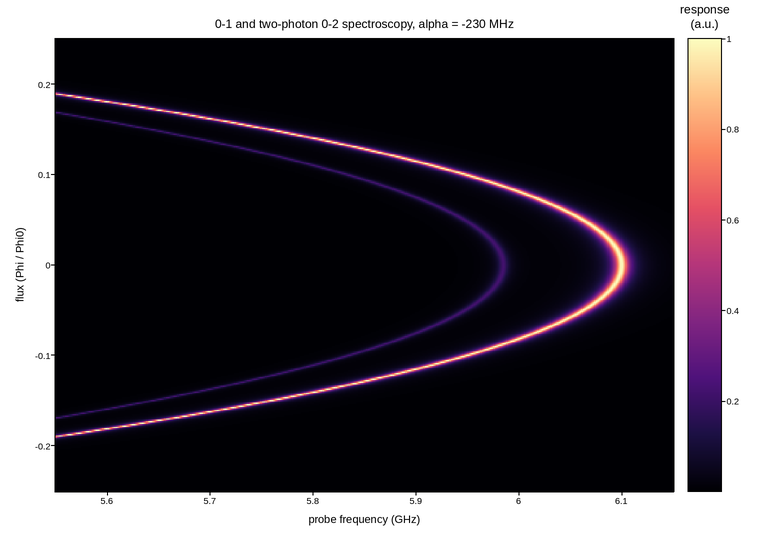
Live figure — pick a tool, then zoom, pan, point-pick or annotate. Nothing is active until a tool is selected.

View this figure’s Vega export ↗ — the raw JSON spec, rendered live by a real Vega engine.

View this figure’s Vega-Lite export ↗ — the raw JSON spec(s), rendered live by a real Vega-Lite engine.

import numpy as np
import polars as pl
import plotpress

F_MAX = 6.10                  # transmon sweet-spot 0-1 frequency, GHz
ALPHA = -0.230                 # anharmonicity, GHz
LINEWIDTH = 0.006              # GHz

frequency = np.linspace(5.55, 6.15, 380)
flux = np.linspace(-0.25, 0.25, 320)
F, PHI = np.meshgrid(frequency, flux)

f01 = F_MAX * np.sqrt(np.abs(np.cos(np.pi * PHI)))
f02_half = f01 + ALPHA / 2.0          # two-photon line: average of 0-1 and 1-2


def lorentzian(detuning, width):
    return width ** 2 / (detuning ** 2 + width ** 2)


response = (lorentzian(F - f01, LINEWIDTH)
            + 0.22 * lorentzian(F - f02_half, LINEWIDTH * 0.8))

# One row per swept (frequency, flux) point -- sorted before the reshape
# below so the pivot back to a grid is correct regardless of row order.
sweep = pl.DataFrame({
    "frequency_ghz": F.ravel(),
    "flux_phi0": PHI.ravel(),
    "response": response.ravel(),
}).sort(["flux_phi0", "frequency_ghz"])

frequency_axis = sweep["frequency_ghz"].unique().sort().to_numpy()
flux_axis = sweep["flux_phi0"].unique().sort().to_numpy()
response = sweep["response"].to_numpy().reshape(flux_axis.size, frequency_axis.size)

fig, ax = plotpress.subplots(figsize=(7.6, 5.4))
mesh = ax.pcolormesh(frequency_axis, flux_axis, response, cmap="magma")
bar = fig.colorbar(mesh, ax=ax)
bar.set_title("response\n(a.u.)")
ax.set_xlabel("probe frequency (GHz)")
ax.set_ylabel("flux (Phi / Phi0)")
ax.set_title(f"0-1 and two-photon 0-2 spectroscopy, alpha = {ALPHA * 1e3:.0f} MHz")
fig.tight_layout()