Readout resonator punch-out

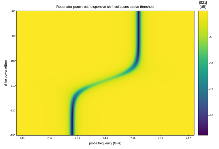
A power sweep of a dispersively coupled readout resonator: transmission against probe frequency and drive power, the calibration that sets the readout operating point.

At low power the resonator responds at its dispersively shifted frequency, pulled by the qubit it is coupled to. Drive it hard enough and the transmon leaves its two lowest levels, the dispersive approximation fails, and the response snaps to the bare cavity frequency – the “punch-out”. The transition is sharp in power and the resonance broadens through it, so the map shows a stepped ridge rather than a smooth drift.

The x axis is frequency and the y axis is drive power in dBm, which is already logarithmic: a sweep spanning 50 dB in power is linear in the plotted coordinate, so no color-scale trickery is needed. The transmission itself is plotted in dB for the same reason.

Live figure — pick a tool, then zoom, pan, point-pick or annotate. Nothing is active until a tool is selected.

View this figure’s Vega export ↗ — the raw JSON spec, rendered live by a real Vega engine.

View this figure’s Vega-Lite export ↗ — the raw JSON spec(s), rendered live by a real Vega-Lite engine.

import numpy as np
import polars as pl
import plotpress

F_DISPERSIVE = 7.128     # low-power (qubit-pulled) frequency (GHz)
F_BARE = 7.152           # bare cavity frequency (GHz)
P_CRIT = -108.0          # punch-out power (dBm)
TRANSITION = 2.2         # width of the punch-out in dB
KAPPA = 0.0011           # loaded linewidth (GHz)

frequency = np.linspace(7.108, 7.172, 380)    # GHz
power = np.linspace(-130.0, -80.0, 320)       # dBm
F, P = np.meshgrid(frequency, power)

# Fraction of the way from dispersive to bare, switching over at P_CRIT.
punched = 1.0 / (1.0 + np.exp(-(P - P_CRIT) / TRANSITION))
center = F_DISPERSIVE + (F_BARE - F_DISPERSIVE) * punched

# The resonance broadens and shallows while it is straddling the transition.
straddle = 4.0 * punched * (1.0 - punched)
width = KAPPA * (1.0 + 2.5 * straddle)
depth = 0.94 * (1.0 - 0.45 * straddle)

transmission = 1.0 - depth * width ** 2 / ((F - center) ** 2 + width ** 2)

# One row per swept (frequency, power) point -- sorted before the reshape
# below so the pivot back to a grid is correct regardless of row order.
sweep = pl.DataFrame({
    "frequency_ghz": F.ravel(),
    "power_dbm": P.ravel(),
    "transmission_db": 20.0 * np.log10(transmission.ravel()),
}).sort(["power_dbm", "frequency_ghz"])

frequency_axis = sweep["frequency_ghz"].unique().sort().to_numpy()
power_axis = sweep["power_dbm"].unique().sort().to_numpy()
transmission_db = sweep["transmission_db"].to_numpy().reshape(power_axis.size, frequency_axis.size)

fig, ax = plotpress.subplots(figsize=(7.6, 5.2))
mesh = ax.pcolormesh(frequency_axis, power_axis, transmission_db, cmap="viridis")
bar = fig.colorbar(mesh, ax=ax)
bar.set_title("|S21|\n(dB)")
ax.set_xlabel("probe frequency (GHz)")
ax.set_ylabel("drive power (dBm)")
ax.set_title("Resonator punch-out: dispersive shift collapses above threshold")
fig.tight_layout()