Flux-tunable transmon spectroscopy

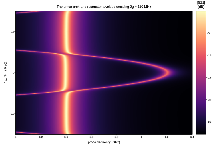
Two-tone spectroscopy of a flux-tunable transmon coupled to a readout resonator: the measured response against probe frequency and applied flux.

The transmon frequency follows the SQUID loop’s flux periodicity,

f_q(Phi) = f_max sqrt(abs(cos(pi Phi / Phi0))),

so it arches down toward zero at half-integer flux quanta. The resonator sits at a fixed f_r, and where the arch crosses it the two hybridize rather than intersect. Diagonalizing the 2x2 Jaynes-Cummings block gives the dressed branches

f_+- = (f_q + f_r)/2 +- sqrt(((f_q - f_r)/2)^2 + g^2),

which repel with a minimum separation of 2g – the avoided crossing that calibrates the coupling.

Both branches must stay legible even though the qubit line is far weaker than the resonator away from the crossing, so the response is plotted in dB. That is a log scale applied to the data rather than to the norm, which suits a quantity already conventionally reported in dB.

Live figure — pick a tool, then zoom, pan, point-pick or annotate. Nothing is active until a tool is selected.

View this figure’s Vega export ↗ — the raw JSON spec, rendered live by a real Vega engine.

View this figure’s Vega-Lite export ↗ — the raw JSON spec(s), rendered live by a real Vega-Lite engine.

import numpy as np
import polars as pl
import plotpress

F_MAX = 6.20             # transmon sweet-spot frequency (GHz)
F_RES = 5.40             # bare resonator frequency (GHz)
COUPLING = 0.055         # g (GHz)
LINEWIDTH = 0.012        # probe linewidth (GHz)

frequency = np.linspace(5.0, 6.4, 380)        # GHz
flux = np.linspace(-0.75, 0.75, 320)          # Phi / Phi0
F, PHI = np.meshgrid(frequency, flux)

f_qubit = F_MAX * np.sqrt(np.abs(np.cos(np.pi * PHI)))

mean = 0.5 * (f_qubit + F_RES)
half_gap = np.sqrt((0.5 * (f_qubit - F_RES)) ** 2 + COUPLING ** 2)
upper, lower = mean + half_gap, mean - half_gap


def lorentzian(detuning, width):
    return width ** 2 / (detuning ** 2 + width ** 2)


# Away from the crossing each branch is mostly one object; the qubit-like branch
# responds far more weakly than the resonator-like one.
mixing = 0.5 * (1.0 + (f_qubit - F_RES) / (2.0 * half_gap))   # qubit weight in upper
weight_upper = 0.12 + 0.88 * (1.0 - mixing)
weight_lower = 0.12 + 0.88 * mixing

response = (weight_upper * lorentzian(F - upper, LINEWIDTH)
            + weight_lower * lorentzian(F - lower, LINEWIDTH))

# One row per swept (frequency, flux) point -- the shape a real two-tone
# spectroscopy sweep is actually logged in, before anything is reshaped for
# plotting. Sorting before the reshape below makes the pivot back to a grid
# correct regardless of what order the sweep happened to log rows in.
sweep = pl.DataFrame({
    "frequency_ghz": F.ravel(),
    "flux_phi0": PHI.ravel(),
    "response_db": 10.0 * np.log10(response.ravel() + 1.5e-3),
}).sort(["flux_phi0", "frequency_ghz"])

frequency_axis = sweep["frequency_ghz"].unique().sort().to_numpy()
flux_axis = sweep["flux_phi0"].unique().sort().to_numpy()
response_db = sweep["response_db"].to_numpy().reshape(flux_axis.size, frequency_axis.size)

fig, ax = plotpress.subplots(figsize=(7.6, 5.2))
mesh = ax.pcolormesh(frequency_axis, flux_axis, response_db, cmap="magma")
bar = fig.colorbar(mesh, ax=ax)
bar.set_title("|S21|\n(dB)")
ax.set_xlabel("probe frequency (GHz)")
ax.set_ylabel("flux (Phi / Phi0)")
ax.set_title(f"Transmon arch and resonator, avoided crossing 2g = {2e3 * COUPLING:.0f} MHz")
fig.tight_layout()