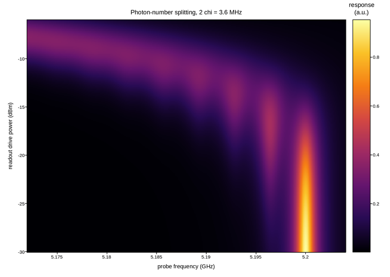
Photon-number splitting of the qubit line

Two-tone qubit spectroscopy while the readout cavity is populated by a continuous drive, swept over probe frequency and that drive’s power. In the dispersive regime each photon in the cavity shifts the qubit transition by 2 chi (the AC Stark shift), so a coherent state with mean photon number n_bar splits the single qubit line into a comb of peaks weighted by the Poisson distribution over n. At low drive power the peaks are few and well separated; raising the power both adds more of them and broadens each one, since photon-number fluctuations dephase the qubit at a rate that itself scales with n_bar – so the comb does not just grow, it washes out into a single broad line at high power, the same “dressed dephasing” that sets a practical ceiling on how hard a dispersive readout can be driven.

Drive power is genuinely logarithmic (dBm), and the mean photon number – linear in drive power – is what is actually swept on an exponential grid along y, which is why the axis is left in dBm rather than converted to a linear power the eye could not use to compare orders of magnitude.

Live figure — pick a tool, then zoom, pan, point-pick or annotate. Nothing is active until a tool is selected.

View this figure’s Vega export ↗ — the raw JSON spec, rendered live by a real Vega engine.

View this figure’s Vega-Lite export ↗ — the raw JSON spec(s), rendered live by a real Vega-Lite engine.

import math

import numpy as np
import polars as pl
import plotpress

F_Q0 = 5.200                # bare qubit frequency, GHz
CHI_MHZ = 1.8                # dispersive shift, MHz
N_MAX = 12                   # photon-number terms to sum

frequency = np.linspace(F_Q0 - 0.028, F_Q0 + 0.004, 380)   # GHz
power_dbm = np.linspace(-30.0, -6.0, 260)
F, P = np.meshgrid(frequency, power_dbm)

n_bar = 50.0 * 10.0 ** (P / 10.0)     # linear photon number from dBm
chi = CHI_MHZ * 1e-3

response = np.zeros_like(F)
for n in range(N_MAX + 1):
    weight = n_bar ** n * np.exp(-n_bar) / math.factorial(n)
    width = 0.0009 + 0.00035 * n_bar    # number-dependent dephasing broadens each peak
    center = F_Q0 - 2.0 * chi * n
    response += weight * width ** 2 / ((F - center) ** 2 + width ** 2)

# One row per swept (frequency, power) point -- sorted before the reshape
# below so the pivot back to a grid is correct regardless of row order.
sweep = pl.DataFrame({
    "frequency_ghz": F.ravel(),
    "power_dbm": P.ravel(),
    "response": response.ravel(),
}).sort(["power_dbm", "frequency_ghz"])

frequency_axis = sweep["frequency_ghz"].unique().sort().to_numpy()
power_axis = sweep["power_dbm"].unique().sort().to_numpy()
response = sweep["response"].to_numpy().reshape(power_axis.size, frequency_axis.size)

fig, ax = plotpress.subplots(figsize=(7.6, 5.4))
mesh = ax.pcolormesh(frequency_axis, power_axis, response, cmap="inferno")
bar = fig.colorbar(mesh, ax=ax)
bar.set_title("response\n(a.u.)")
ax.set_xlabel("probe frequency (GHz)")
ax.set_ylabel("readout drive power (dBm)")
ax.set_title(f"Photon-number splitting, 2 chi = {2 * CHI_MHZ:.1f} MHz")
fig.tight_layout()