Single-shot readout fidelity optimization

Assignment fidelity of single-shot dispersive readout, swept over probe frequency and integration time – the calibration that sets a superconducting qubit’s actual operating readout point, not just its resonator’s bare frequency. Two competing effects shape the map: fidelity needs enough signal to noise to separate the two states, which grows with both how close the probe sits to the frequency of maximum dispersive contrast and how long the integration window is; but a long integration window also gives the qubit more time to relax mid-measurement, misclassifying a decayed |1> as |0>. The result is a genuine two-dimensional optimum – an island of high fidelity at a finite integration time, not a monotonic climb – that neither a frequency sweep nor a duration sweep alone would reveal.

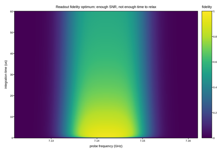
Live figure — pick a tool, then zoom, pan, point-pick or annotate. Nothing is active until a tool is selected.

View this figure’s Vega export ↗ — the raw JSON spec, rendered live by a real Vega engine.

View this figure’s Vega-Lite export ↗ — the raw JSON spec(s), rendered live by a real Vega-Lite engine.

import numpy as np
import polars as pl
import plotpress

F_OPT = 7.142                # GHz, frequency of maximum dispersive contrast
CONTRAST_WIDTH = 0.006        # GHz
SNR_MAX = 3.2                  # SNR reached at long integration, on resonance
T1_QUBIT = 25.0                 # microseconds
T_SNR = 0.35                   # microseconds, integration time to reach half SNR_MAX

frequency = np.linspace(F_OPT - 0.02, F_OPT + 0.02, 320)
duration = np.linspace(0.02, 60.0, 280)        # microseconds
F, T = np.meshgrid(frequency, duration)

contrast = np.exp(-0.5 * ((F - F_OPT) / CONTRAST_WIDTH) ** 2)
snr = SNR_MAX * contrast * np.sqrt(T / (T + T_SNR))
p_decay_during_readout = 1.0 - np.exp(-T / T1_QUBIT)   # chance |1> relaxed mid-shot

fidelity = (1.0 - np.exp(-snr ** 2 / 2.0)) * (1.0 - 0.5 * p_decay_during_readout)

# One row per swept (frequency, duration) point -- sorted before the reshape
# below so the pivot back to a grid is correct regardless of row order.
sweep = pl.DataFrame({
    "frequency_ghz": F.ravel(),
    "duration_us": T.ravel(),
    "fidelity": fidelity.ravel(),
}).sort(["duration_us", "frequency_ghz"])

frequency_axis = sweep["frequency_ghz"].unique().sort().to_numpy()
duration_axis = sweep["duration_us"].unique().sort().to_numpy()
fidelity = sweep["fidelity"].to_numpy().reshape(duration_axis.size, frequency_axis.size)

fig, ax = plotpress.subplots(figsize=(7.6, 5.2))
mesh = ax.pcolormesh(frequency_axis, duration_axis, fidelity, cmap="viridis", vmin=0.0, vmax=1.0)
bar = fig.colorbar(mesh, ax=ax)
bar.set_title("fidelity")
ax.set_xlabel("probe frequency (GHz)")
ax.set_ylabel("integration time (us)")
ax.set_title("Readout fidelity optimum: enough SNR, not enough time to relax")
fig.tight_layout()