Reflectance contrast vs gate voltage

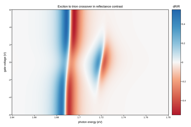
Gate-dependent reflectance contrast dR/R of a monolayer semiconductor – the standard way to watch excitons convert to trions as carriers are added electrostatically.

At charge neutrality the neutral exciton X0 dominates. Doping either way transfers oscillator strength to a charged exciton roughly 30 meV below it: X+ for holes, X- for electrons. Both resonances also blue-shift slightly as the Fermi level rises.

Reflectance contrast is measured against a bare-substrate reference, so each resonance appears as a dispersive lineshape – positive on one side of the resonance and negative on the other – and the data is genuinely signed. That calls for a diverging colormap with limits placed symmetrically about zero, so that dR/R = 0 lands on the neutral midpoint instead of drifting to whatever color the autoscaled range happens to put there.

Live figure — pick a tool, then zoom, pan, point-pick or annotate. Nothing is active until a tool is selected.

View this figure’s Vega export ↗ — the raw JSON spec, rendered live by a real Vega engine.

View this figure’s Vega-Lite export ↗ — the raw JSON spec(s), rendered live by a real Vega-Lite engine.

import numpy as np
import polars as pl
import plotpress

X0_ENERGY = 1.720        # neutral exciton (eV)
TRION_BINDING = 0.030    # trion sits this far below X0 (eV)
LINEWIDTH = 0.005        # half-width (eV)

energy = np.linspace(1.64, 1.78, 360)         # eV
gate = np.linspace(-6.0, 6.0, 300)            # V
E, VG = np.meshgrid(energy, gate)


def dispersive(detuning, width):
    """Derivative-of-Lorentzian lineshape.

    Reflectance contrast from a thin film is dispersive -- positive on one side
    of the resonance, negative on the other. This form falls off as
    ``1/detuning^3`` rather than ``1/detuning``, so neighbouring resonances stay
    distinct instead of drowning the map in their tails.
    """
    x = detuning / width
    return -2.0 * x / (1.0 + x ** 2) ** 2


# Doping rises with |Vg|; electrons for Vg > 0, holes for Vg < 0.
electron = 1.0 / (1.0 + np.exp(-(VG - 1.0) / 0.8))
hole = 1.0 / (1.0 + np.exp((VG + 1.0) / 0.8))
neutral = 1.0 - electron - hole

# Band-gap renormalization plus Pauli blocking shifts both peaks with doping.
shift = 0.004 * np.tanh(VG / 3.0)
x0 = X0_ENERGY + shift
trion = X0_ENERGY - TRION_BINDING + 0.6 * shift

signal = (np.clip(neutral, 0.0, None) * dispersive(E - x0, LINEWIDTH)
          + 0.85 * electron * dispersive(E - trion, LINEWIDTH * 1.2)
          + 0.75 * hole * dispersive(E - trion, LINEWIDTH * 1.2))

# One row per swept (energy, gate) point -- sorted before the reshape below
# so the pivot back to a grid is correct regardless of row order.
sweep = pl.DataFrame({
    "energy_ev": E.ravel(),
    "gate_v": VG.ravel(),
    "signal": signal.ravel(),
}).sort(["gate_v", "energy_ev"])

energy_axis = sweep["energy_ev"].unique().sort().to_numpy()
gate_axis = sweep["gate_v"].unique().sort().to_numpy()
signal = sweep["signal"].to_numpy().reshape(gate_axis.size, energy_axis.size)
lim = float(sweep["signal"].abs().max())

fig, ax = plotpress.subplots(figsize=(7.5, 5.0))
mesh = ax.pcolormesh(energy_axis, gate_axis, signal, cmap="RdBu", vmin=-lim, vmax=lim)
bar = fig.colorbar(mesh, ax=ax)
bar.set_title("dR/R")
ax.set_xlabel("photon energy (eV)")
ax.set_ylabel("gate voltage (V)")
ax.set_title("Exciton to trion crossover in reflectance contrast")
fig.tight_layout()