Tunneling spectroscopy of a Majorana device

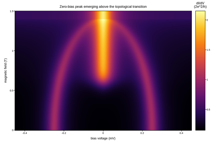
Differential conductance dI/dV of a proximitized nanowire, swept over bias voltage and applied magnetic field – the measurement used to look for Majorana bound states at the wire ends.

Three features share one map, which is why the color scale has to accommodate all of them at once. The induced gap follows Delta(B) = Delta0 sqrt(1 - (B/Bc)^2), so the coherence peaks at +/- Delta move inward and close near Bc. Above a topological transition at B* a zero-bias peak switches on and then persists as a flat ridge at V = 0, which is the signature of interest.

Conductance is strictly positive and the zero-bias peak is several times the sub-gap background, so a sequential map with autoscaled limits reads correctly; a diverging map would falsely imply a meaningful zero.

The physics here is a caricature – a real device would show finite-temperature broadening, disorder, and quasiparticle states in the gap – but it is the shape of the plot that matters for the example.

Live figure — pick a tool, then zoom, pan, point-pick or annotate. Nothing is active until a tool is selected.

View this figure’s Vega export ↗ — the raw JSON spec, rendered live by a real Vega engine.

View this figure’s Vega-Lite export ↗ — the raw JSON spec(s), rendered live by a real Vega-Lite engine.

import numpy as np
import polars as pl
import plotpress

DELTA0 = 0.25            # induced gap at zero field (meV)
B_CRIT = 1.4             # field where the gap closes (T)
B_STAR = 0.60            # topological transition (T)
WIDTH = 0.035            # peak half-width (meV)

bias = np.linspace(-0.45, 0.45, 340)          # mV
field = np.linspace(0.0, 1.5, 260)            # T
V, B = np.meshgrid(bias, field)


def lorentzian(x, width):
    return width ** 2 / (x ** 2 + width ** 2)


gap = DELTA0 * np.sqrt(np.clip(1.0 - (B / B_CRIT) ** 2, 0.0, None))

# Coherence peaks at +/- Delta(B), fading as the gap closes.
weight = np.clip(gap / DELTA0, 0.0, 1.0)
coherence = 0.9 * weight * (lorentzian(V - gap, WIDTH) + lorentzian(V + gap, WIDTH))

# Zero-bias peak: switches on at B* and stays pinned to V = 0.
turn_on = 1.0 / (1.0 + np.exp(-(B - B_STAR) / 0.05))
zero_bias = 1.6 * turn_on * lorentzian(V, WIDTH * 1.3)

# Sub-gap background fills in as the gap closes.
background = 0.12 + 0.35 * (1.0 - weight)

conductance = background + coherence + zero_bias

# One row per swept (bias, field) point -- sorted before the reshape below so
# the pivot back to a grid is correct regardless of row order.
sweep = pl.DataFrame({
    "bias_mv": V.ravel(),
    "field_t": B.ravel(),
    "conductance": conductance.ravel(),
}).sort(["field_t", "bias_mv"])

bias_axis = sweep["bias_mv"].unique().sort().to_numpy()
field_axis = sweep["field_t"].unique().sort().to_numpy()
conductance = sweep["conductance"].to_numpy().reshape(field_axis.size, bias_axis.size)

fig, ax = plotpress.subplots(figsize=(7.5, 5.0))
mesh = ax.pcolormesh(bias_axis, field_axis, conductance, cmap="inferno")
bar = fig.colorbar(mesh, ax=ax)
bar.set_title("dI/dV\n(2e^2/h)")
ax.set_xlabel("bias voltage (mV)")
ax.set_ylabel("magnetic field (T)")
ax.set_title("Zero-bias peak emerging above the topological transition")
fig.tight_layout()