Double-dot charge stability diagram

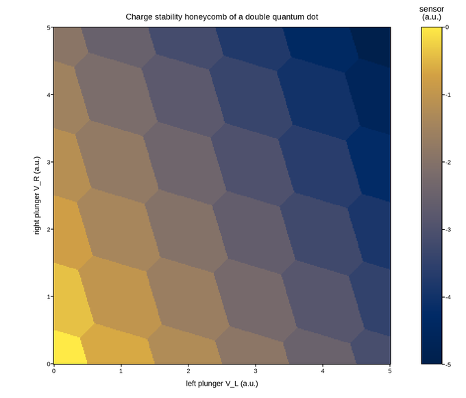
The honeycomb map that defines a semiconductor spin-qubit device: charge-sensor signal against the two plunger-gate voltages, with each cell a fixed electron occupation (N_L, N_R) of the double dot.

For every gate setting the dot settles into whichever integer occupation minimizes the electrostatic energy,

E = (1/2) Ec_L N_L^2 + (1/2) Ec_R N_R^2 + Ecm N_L N_R

• N_L (a_LL V_L + a_LR V_R) - N_R (a_RL V_L + a_RR V_R),

so the field is piecewise constant with sharp boundaries where the ground state switches. The mutual charging energy Ecm is what splits the crossings into the characteristic honeycomb vertices rather than a simple square grid.

This one is a stress test for a mesh renderer rather than for a color scale: the data is flat plateaus separated by one-cell discontinuities, so any smoothing or interpolation would blur exactly the boundaries the measurement is about. pcolormesh maps one cell to one cell, and the plateau edges stay sharp.

Live figure — pick a tool, then zoom, pan, point-pick or annotate. Nothing is active until a tool is selected.

View this figure’s Vega export ↗ — the raw JSON spec, rendered live by a real Vega engine.

View this figure’s Vega-Lite export ↗ — the raw JSON spec(s), rendered live by a real Vega-Lite engine.

import numpy as np
import polars as pl
import plotpress

EC_L, EC_R, EC_M = 1.0, 1.0, 0.28      # charging energies (arbitrary units)
A_LL, A_LR = 1.0, 0.30                 # gate-to-dot lever arms
A_RL, A_RR = 0.30, 1.0
N_MAX = 6                              # occupations considered per dot

v_left = np.linspace(0.0, 5.0, 340)
v_right = np.linspace(0.0, 5.0, 340)
VL, VR = np.meshgrid(v_left, v_right)

# Energy of every candidate (N_L, N_R), then keep the lowest at each gate point.
occupations = [(nl, nr) for nl in range(N_MAX + 1) for nr in range(N_MAX + 1)]
energies = np.stack([
    0.5 * EC_L * nl ** 2 + 0.5 * EC_R * nr ** 2 + EC_M * nl * nr
    - nl * (A_LL * VL + A_LR * VR) - nr * (A_RL * VL + A_RR * VR)
    for nl, nr in occupations
])
ground = np.argmin(energies, axis=0)

n_left = np.array([o[0] for o in occupations])[ground]
n_right = np.array([o[1] for o in occupations])[ground]

# A nearby charge sensor couples more strongly to the left dot than the right.
sensor = -(0.62 * n_left + 0.38 * n_right)

# One row per swept (V_L, V_R) gate point -- sorted before the reshape below
# so the pivot back to a grid is correct regardless of row order.
sweep = pl.DataFrame({
    "v_left": VL.ravel(),
    "v_right": VR.ravel(),
    "sensor": sensor.ravel(),
}).sort(["v_right", "v_left"])

v_left_axis = sweep["v_left"].unique().sort().to_numpy()
v_right_axis = sweep["v_right"].unique().sort().to_numpy()
sensor = sweep["sensor"].to_numpy().reshape(v_right_axis.size, v_left_axis.size)

fig, ax = plotpress.subplots(figsize=(6.8, 5.8))
mesh = ax.pcolormesh(v_left_axis, v_right_axis, sensor, cmap="cividis")
bar = fig.colorbar(mesh, ax=ax)
bar.set_title("sensor\n(a.u.)")
ax.set_aspect("equal")
ax.set_xlabel("left plunger V_L (a.u.)")
ax.set_ylabel("right plunger V_R (a.u.)")
ax.set_title("Charge stability honeycomb of a double quantum dot")
fig.tight_layout()