Single-qubit gate speed limit: Rabi map with a leakage threshold overlaid

Excited-state population from a driven Rabi oscillation on resonance, swept over both drive amplitude and pulse duration rather than the more usual amplitude/detuning or detuning/duration chevron – the map a “how fast can this gate go” calibration actually needs, since amplitude and duration trade off directly against each other to hit exactly a pi pulse, Omega * t = pi. That trade-off is not free: leakage into the second excited state grows with drive amplitude relative to the qubit’s anharmonicity, so pushing the gate faster by raising the amplitude along that same pi-pulse ridge eventually crosses into leaky territory. The contour marks a 1% leakage threshold directly on the Rabi map, so the usable pi-pulse condition – fast, complete, and leakage-free – is read off as wherever the ridge sits before it crosses the contour, not from a separate figure.

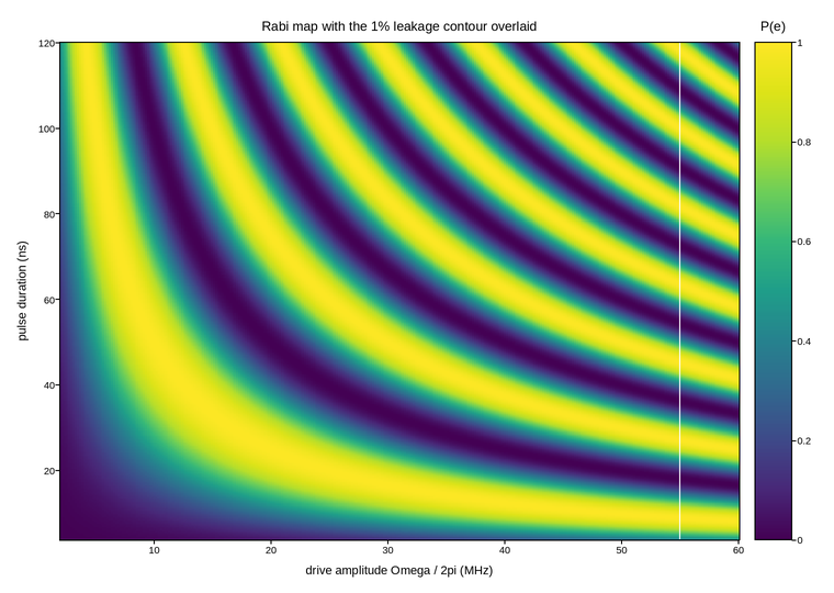
Live figure — pick a tool, then zoom, pan, point-pick or annotate. Nothing is active until a tool is selected.

View this figure’s Vega export ↗ — the raw JSON spec, rendered live by a real Vega engine.

View this figure’s Vega-Lite export ↗ — the raw JSON spec(s), rendered live by a real Vega-Lite engine.

import numpy as np
import polars as pl
import plotpress

ANHARMONICITY_MHZ = 220.0      # |alpha|, sets the leakage scale
LEAKAGE_COEFF = 0.16            # dimensionless prefactor on (Omega/alpha)^2

amplitude = np.linspace(2.0, 60.0, 320)       # Omega / 2pi, MHz
duration = np.linspace(4.0, 120.0, 300)        # ns
OMEGA_MHZ, T = np.meshgrid(amplitude, duration)

omega = 2.0 * np.pi * OMEGA_MHZ * 1e-3        # rad/ns
p_excited = np.sin(omega * T / 2.0) ** 2

leakage = LEAKAGE_COEFF * (OMEGA_MHZ / ANHARMONICITY_MHZ) ** 2

# One row per swept (amplitude, duration) point -- sorted before the reshape
# below so the pivot back to a grid is correct regardless of row order.
sweep = pl.DataFrame({
    "amplitude_mhz": OMEGA_MHZ.ravel(),
    "duration_ns": T.ravel(),
    "p_excited": p_excited.ravel(),
    "leakage": leakage.ravel(),
}).sort(["duration_ns", "amplitude_mhz"])

amplitude_axis = sweep["amplitude_mhz"].unique().sort().to_numpy()
duration_axis = sweep["duration_ns"].unique().sort().to_numpy()
p_excited = sweep["p_excited"].to_numpy().reshape(duration_axis.size, amplitude_axis.size)
leakage = sweep["leakage"].to_numpy().reshape(duration_axis.size, amplitude_axis.size)

fig, ax = plotpress.subplots(figsize=(7.6, 5.4))
mesh = ax.pcolormesh(amplitude_axis, duration_axis, p_excited, cmap="viridis", vmin=0.0, vmax=1.0)
bar = fig.colorbar(mesh, ax=ax)
bar.set_title("P(e)")
ax.contour(amplitude_axis, duration_axis, leakage, levels=[0.01], colors="white")
ax.set_xlabel("drive amplitude Omega / 2pi (MHz)")
ax.set_ylabel("pulse duration (ns)")
ax.set_title("Rabi map with the 1% leakage contour overlaid")
fig.tight_layout()