T1 relaxation vs frequency and time: wandering TLS defects

Repeated T1 measurements across a tunable transmon’s accessible frequency range, stacked over several hours. Superconducting qubits couple to stray two-level systems (TLS) living in the amorphous oxides of the junction and substrate; wherever a TLS’s own resonance lines up with the qubit frequency, relaxation speeds up and T1 drops. The feature that marks a TLS, rather than some other loss mechanism, is that its resonance frequency drifts slowly over hours as the defect’s local environment relaxes – so repeating the same frequency sweep on a cadence of minutes and stacking the results in time turns a single narrow T1 dip into a wandering dark streak instead of a fixed one.

A sequential colormap is the right choice for T1 itself – there is no meaningful zero-crossing, only “worse” and “better” – but the map is really being read for its dark features, the TLS streaks, rather than its absolute color, which is why a colormap dark at low values earns its place here rather than something brighter across the whole range.

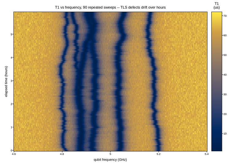
Live figure — pick a tool, then zoom, pan, point-pick or annotate. Nothing is active until a tool is selected.

View this figure’s Vega export ↗ — the raw JSON spec, rendered live by a real Vega engine.

View this figure’s Vega-Lite export ↗ — the raw JSON spec(s), rendered live by a real Vega-Lite engine.

import numpy as np
import polars as pl
import plotpress

T1_BASELINE = 65.0        # microseconds, away from any TLS
N_TLS = 6
rng = np.random.default_rng(77)

frequency = np.linspace(4.6, 5.4, 300)      # GHz, swept via flux each cycle
n_sweeps = 90
elapsed = np.arange(n_sweeps) * 4.0 / 60.0  # hours, one sweep every 4 minutes

# Each TLS starts at a random frequency and undergoes slow spectral diffusion
# (a random walk) over the measurement -- physically, its own local
# environment relaxing between sweeps.
tls_freq0 = rng.uniform(frequency[0] + 0.05, frequency[-1] - 0.05, N_TLS)
tls_drift = np.cumsum(rng.normal(0.0, 0.0026, (n_sweeps, N_TLS)), axis=0)
tls_freq = tls_freq0[None, :] + tls_drift                  # (n_sweeps, N_TLS)
tls_coupling = rng.uniform(0.006, 0.020, N_TLS)             # GHz, dip strength
tls_width = rng.uniform(0.0015, 0.004, N_TLS)               # GHz, dip width

F, ELAPSED = np.meshgrid(frequency, elapsed)
rate = np.full_like(F, 1.0 / T1_BASELINE)
for i in range(N_TLS):
    detuning = F - tls_freq[:, i][:, None]
    rate += tls_coupling[i] ** 2 / (detuning ** 2 + tls_width[i] ** 2) / T1_BASELINE
T1_map = 1.0 / rate
T1_map *= 1.0 + rng.normal(0.0, 0.03, T1_map.shape)    # measurement scatter
T1_map = np.clip(T1_map, 1.0, None)

# One row per (frequency, sweep time) point -- sorted before the reshape
# below so the pivot back to a grid is correct regardless of row order.
sweeps = pl.DataFrame({
    "frequency_ghz": F.ravel(),
    "elapsed_hours": ELAPSED.ravel(),
    "t1_us": T1_map.ravel(),
}).sort(["elapsed_hours", "frequency_ghz"])

frequency_axis = sweeps["frequency_ghz"].unique().sort().to_numpy()
elapsed_axis = sweeps["elapsed_hours"].unique().sort().to_numpy()
T1_map = sweeps["t1_us"].to_numpy().reshape(elapsed_axis.size, frequency_axis.size)

fig, ax = plotpress.subplots(figsize=(7.6, 5.4))
mesh = ax.pcolormesh(frequency_axis, elapsed_axis, T1_map, cmap="cividis")
bar = fig.colorbar(mesh, ax=ax)
bar.set_title("T1\n(us)")
ax.set_xlabel("qubit frequency (GHz)")
ax.set_ylabel("elapsed time (hours)")
ax.set_title(f"T1 vs frequency, {n_sweeps} repeated sweeps -- TLS defects drift over hours")
fig.tight_layout()