Dose-response curves and EC50

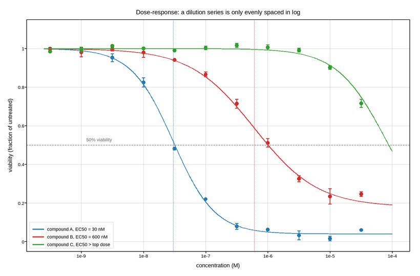
Cell viability against drug concentration for three compounds. Concentration is prepared as a dilution series – each step a fixed multiple of the last – so the doses are evenly spaced in the logarithm and nowhere else. On a linear axis the eight lowest doses would pile up against the origin and the curve would look like a step; set_xscale("log") restores the even spacing the experiment was designed around, and turns the sigmoid into the symmetric shape the Hill equation predicts.

That symmetry is the point. EC50 is read off where the fitted curve crosses the midpoint between the upper and lower plateaus, and a plateau is only identifiable if the dose range extends past it on both sides – which is why weak compounds whose curve has not levelled off are flagged rather than quoted.

The replicate error bars are drawn as the standard error of three wells per dose. They are widest in the middle of the transition, which is the usual pattern and a reason EC50 estimates are less precise than the tidy fitted curve suggests.

Live figure — pick a tool, then zoom, pan, point-pick or annotate. Nothing is active until a tool is selected.

View this figure’s Vega export ↗ — the raw JSON spec, rendered live by a real Vega engine.

View this figure’s Vega-Lite export ↗ — the raw JSON spec(s), rendered live by a real Vega-Lite engine.

import numpy as np
import polars as pl
import plotpress

rng = np.random.default_rng(404)

doses = 10.0 ** np.arange(-9.5, -4.0, 0.5)        # molar, half-log dilutions
fine = 10.0 ** np.linspace(-9.6, -4.0, 400)

COMPOUNDS = [
    # name,        EC50 (M), Hill slope, bottom plateau, colour
    ("compound A", 3.0e-8, 1.30, 0.04, "#1f77b4"),
    ("compound B", 6.0e-7, 0.85, 0.18, "#d62728"),
    ("compound C", 8.0e-5, 1.10, 0.05, "#2ca02c"),   # EC50 beyond the top dose
]


def hill(c, ec50, slope, bottom, top=1.0):
    return bottom + (top - bottom) / (1.0 + (c / ec50) ** slope)


fig, ax = plotpress.subplots(figsize=(8.2, 5.4))

for name, ec50, slope, bottom, color in COMPOUNDS:
    truth = hill(doses, ec50, slope, bottom)
    # Three wells per dose; noise peaks mid-transition where the slope is
    # steepest, so a small pipetting error moves the reading the most.
    spread = 0.02 + 0.10 * truth * (1.0 - truth)
    wells = truth[:, None] + rng.normal(0.0, spread[:, None], (doses.size, 3))

    # One row per well -- the shape a plate reader's own raw output is in,
    # before triplicate wells are aggregated into a mean and standard error.
    plate = pl.DataFrame({"dose": np.repeat(doses, 3), "viability": wells.ravel()})
    stats = plate.group_by("dose", maintain_order=True).agg(
        pl.col("viability").mean().alias("mean"),
        (pl.col("viability").std(ddof=1) / np.sqrt(3)).alias("sem"),
    )
    mean = stats["mean"].to_numpy()
    sem = stats["sem"].to_numpy()

    covered = ec50 < doses.max()
    ax.errorbar(doses, mean, yerr=sem, color=color, marker="o", markersize=5.0,
                linestyle="none", capsize=3.0,
                label=(f"{name}, EC50 = {ec50 * 1e9:.0f} nM" if covered
                       else f"{name}, EC50 > top dose"))
    ax.plot(fine, hill(fine, ec50, slope, bottom), color=color, linewidth=1.6,
            alpha=0.9)
    if covered:
        ax.axvline(ec50, color=color, linestyle=":", linewidth=1.0, alpha=0.8)

ax.axhline(0.5, color="#888888", linestyle="--", linewidth=1.0)
ax.text(1.2e-9, 0.52, "50% viability", fontsize=9, color="#666666")

ax.set_xscale("log")
ax.set_ylim(-0.05, 1.15)
ax.set_xlabel("concentration (M)")
ax.set_ylabel("viability (fraction of untreated)")
ax.set_title("Dose-response: a dilution series is only evenly spaced in log")
ax.legend(loc="lower left")
ax.grid(True)
fig.tight_layout()