ECG rhythm strip with beat annotations

Six seconds of a single-lead electrocardiogram, drawn the way a monitor prints it. Almost every choice here is a clinical convention rather than a graphical preference, and getting them wrong makes the trace unreadable to the people who read traces.

The x axis is seconds and the y axis is millivolts, but the aspect is the specification: ECG paper is 25 mm/s by 10 mm/mV, so one second of time and one millivolt of amplitude occupy a fixed physical ratio – 10/25, or 0.4. set_aspect(0.4) fixes that ratio in data units, which is what makes an ST elevation measurable by eye rather than a function of how wide the browser window happens to be. It also dictates the figure’s shape: a strip six seconds long and two millivolts tall is seven times wider than it is high, and choosing figsize to match is what keeps the fixed aspect from leaving a band of empty canvas above and below the trace.

Rhythm is diagnosed from the spacing of R peaks, not from their shape, so the detected peaks are marked and the instantaneous heart rate derived from each R-R interval is annotated. This strip contains one premature ventricular contraction – an early, wide, oppositely-deflected beat followed by a compensatory pause – which is exactly the event the R-R annotation exists to make obvious.

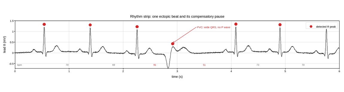
Live figure — pick a tool, then zoom, pan, point-pick or annotate. Nothing is active until a tool is selected.

View this figure’s Vega export ↗ — the raw JSON spec, rendered live by a real Vega engine.

View this figure’s Vega-Lite export ↗ — the raw JSON spec(s), rendered live by a real Vega-Lite engine.

import numpy as np
import polars as pl
import plotpress

rng = np.random.default_rng(60)

FS = 500.0                                        # samples per second
DURATION = 6.0
t = np.arange(0.0, DURATION, 1.0 / FS)


def gaussian(t, centre, amp, width):
    return amp * np.exp(-((t - centre) ** 2) / (2.0 * width ** 2))


def normal_beat(t, onset):
    """P wave, sharp QRS complex, broad T wave -- in millivolts."""
    return (gaussian(t, onset + 0.00, 0.13, 0.022)      # P
            + gaussian(t, onset + 0.16, -0.10, 0.008)   # Q
            + gaussian(t, onset + 0.19, 1.15, 0.009)    # R
            + gaussian(t, onset + 0.22, -0.22, 0.010)   # S
            + gaussian(t, onset + 0.42, 0.28, 0.038))   # T


def ectopic_beat(t, onset):
    """A PVC: no P wave, wide QRS, and a T wave opposite to the QRS."""
    return (gaussian(t, onset + 0.18, -0.75, 0.030)
            + gaussian(t, onset + 0.26, 0.35, 0.045)
            + gaussian(t, onset + 0.46, 0.30, 0.070))


# Sinus rhythm near 72 bpm with a little respiratory sinus arrhythmia, one
# ectopic beat that arrives early, and the compensatory pause that follows it.
onsets, kinds, clock = [], [], 0.35
while clock < DURATION - 0.6:
    onsets.append(clock)
    kinds.append("N")
    clock += 0.833 + 0.035 * np.sin(2 * np.pi * clock / 4.0)
onsets[3], kinds[3] = onsets[3] - 0.24, "V"        # premature
for i in range(4, len(onsets)):
    onsets[i] += 0.20                              # compensatory pause

ecg = np.zeros_like(t)
for onset, kind in zip(onsets, kinds):
    ecg += (ectopic_beat if kind == "V" else normal_beat)(t, onset)

# Baseline wander from respiration, plus mains hum and electrode noise.
ecg += 0.06 * np.sin(2 * np.pi * 0.28 * t)
ecg += 0.008 * np.sin(2 * np.pi * 50.0 * t)
ecg += rng.normal(0.0, 0.011, t.size)

# One row per sample -- the shape a monitor's own lead export is in, before
# R peaks are detected and beat-to-beat intervals are derived from it.
strip = pl.DataFrame({"time": t, "lead_ii": ecg})
t = strip["time"].to_numpy()
ecg = strip["lead_ii"].to_numpy()

r_times = np.array([o + (0.26 if k == "V" else 0.19)
                    for o, k in zip(onsets, kinds)])
r_amps = np.array([np.max(ecg[(t > rt - 0.03) & (t < rt + 0.03)]) for rt in r_times])
rr = np.diff(r_times)

fig, ax = plotpress.subplots(figsize=(11.5, 3.1))
ax.plot(t, ecg, color="#111111", linewidth=0.9)
ax.scatter(r_times, r_amps + 0.13, s=7.0, color="#d62728",
           label="detected R peak")

for i, interval in enumerate(rr):
    mid = 0.5 * (r_times[i] + r_times[i + 1])
    ax.text(mid, -0.60, f"{60.0 / interval:.0f}", ha="center", fontsize=8,
            color="#d62728" if interval < 0.70 or interval > 0.95 else "#666666")
ax.text(0.04, -0.60, "bpm", ha="left", fontsize=8, color="#666666")

ax.annotate("PVC: wide QRS, no P wave", xy=(r_times[3], r_amps[3] + 0.16),
            xytext=(r_times[3] + 0.45, 1.15), arrowprops={"color": "#d62728"},
            color="#d62728", fontsize=9)

ax.set_aspect(0.4)                                 # 25 mm/s by 10 mm/mV
ax.set_xlim(0.0, DURATION)
ax.set_ylim(-0.72, 1.50)
ax.set_xlabel("time (s)")
ax.set_ylabel("lead II (mV)")
ax.set_title("Rhythm strip: one ectopic beat and its compensatory pause")
ax.legend(loc="upper right")
ax.grid(True)
fig.tight_layout()