Calcium imaging population raster

Two-photon calcium imaging of a cortical population: each row is one neuron’s fluorescence expressed as dF/F, the fractional change against that cell’s own baseline. Sorting the rows by response latency turns a population recording into a picture of sequential recruitment.

dF/F is signed. A calcium transient is a sharp positive excursion with a slow decay, but inhibited cells and baseline drift push traces below their own resting fluorescence, and those negative deflections are real physiology rather than noise to be clipped. The map is therefore diverging with limits symmetric about zero, so a quiescent cell sits at the neutral midpoint and suppression stays distinguishable from silence.

The stimulus arrives at t = 2 s; the recruitment sweep after it is what the sort makes visible.

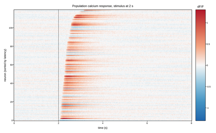
Live figure — pick a tool, then zoom, pan, point-pick or annotate. Nothing is active until a tool is selected.

View this figure’s Vega export ↗ — the raw JSON spec, rendered live by a real Vega engine.

View this figure’s Vega-Lite export ↗ — the raw JSON spec(s), rendered live by a real Vega-Lite engine.

import numpy as np
import polars as pl
import plotpress

rng = np.random.default_rng(37)
N_CELLS = 120
time = np.linspace(0.0, 8.0, 400)          # s
cells = np.arange(N_CELLS)

STIM_T = 2.0
TAU_RISE, TAU_DECAY = 0.08, 0.65           # GCaMP-like kinetics

latency = np.sort(rng.gamma(2.2, 0.16, N_CELLS))     # sorted, so the sweep shows
amplitude = rng.gamma(3.0, 0.22, N_CELLS)
suppressed = rng.random(N_CELLS) < 0.18              # inhibited subpopulation
amplitude[suppressed] *= -0.45

T = time[None, :]
onset = STIM_T + latency[:, None]
dt = np.clip(T - onset, 0.0, None)
trace = amplitude[:, None] * (1.0 - np.exp(-dt / TAU_RISE)) * np.exp(-dt / TAU_DECAY)
trace *= (T >= onset)

# Slow baseline drift, each cell with its own phase, plus shot noise.
drift = 0.05 * np.sin(2.0 * np.pi * (T / 11.0 + rng.random((N_CELLS, 1))))
dff = trace + drift + rng.normal(0.0, 0.025, trace.shape)

# One row per (cell, time sample) recording -- the shape a two-photon
# acquisition's own trace export is in, before it is gridded for the mesh.
CELL, TIME = np.meshgrid(cells, time, indexing="ij")
recording = pl.DataFrame({"cell": CELL.ravel(), "time": TIME.ravel(), "dff": dff.ravel()}) \
    .sort(["cell", "time"])
cells = recording["cell"].unique().sort().to_numpy()
time = recording["time"].unique().sort().to_numpy()
dff = recording["dff"].to_numpy().reshape(cells.size, time.size)

lim = float(np.abs(dff).max())
fig, ax = plotpress.subplots(figsize=(8.4, 5.2))
mesh = ax.pcolormesh(time, cells, dff, cmap="RdBu_r", vmin=-lim, vmax=lim)
fig.colorbar(mesh, ax=ax).set_title("dF/F")
ax.axvline(STIM_T, color="#000000", linestyle="--", linewidth=1.2)
ax.set_xlabel("time (s)")
ax.set_ylabel("neuron (sorted by latency)")
ax.set_title("Population calcium response, stimulus at 2 s")
fig.tight_layout()