OCT retinal cross-section

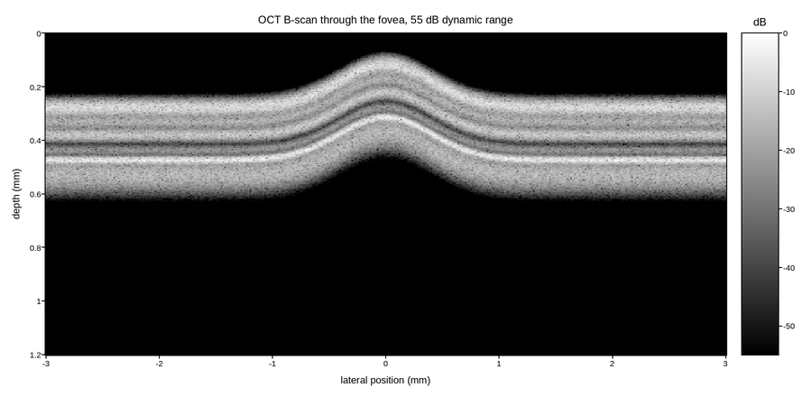
Optical coherence tomography builds a depth profile from the interference between light returned by tissue and a reference arm, then sweeps the beam laterally – so a B-scan arrives as backscatter intensity against lateral position and depth. It is the routine imaging test in ophthalmology because the retina’s layers separate cleanly in it.

Backscatter spans four or five decades between the highly reflective retinal pigment epithelium and the near-transparent vitreous, so OCT is displayed in dB, log-compressed exactly like ultrasound. The log lives in the data and the colour norm stays linear over dB.

The layers are the diagnosis: nerve fibre layer at the top, the dark band of photoreceptor inner segments, then the bright RPE and choroid beneath. The foveal pit dips through the middle.

Live figure — pick a tool, then zoom, pan, point-pick or annotate. Nothing is active until a tool is selected.

View this figure’s Vega export ↗ — the raw JSON spec, rendered live by a real Vega engine.

View this figure’s Vega-Lite export ↗ — the raw JSON spec(s), rendered live by a real Vega-Lite engine.

import numpy as np
import polars as pl
import plotpress

rng = np.random.default_rng(17)
lateral = np.linspace(-3.0, 3.0, 380)      # mm
depth = np.linspace(0.0, 1.2, 300)         # mm
X, Z = np.meshgrid(lateral, depth)

# Foveal pit: the inner layers thin toward the centre.
pit = 0.16 * np.exp(-(X ** 2) / 0.34)
surface = 0.26 - pit

signal = np.full_like(X, 4.0e-4)           # vitreous: almost no return
LAYERS = [(0.000, 0.035, 0.55),            # nerve fibre layer
          (0.055, 0.030, 0.22),            # inner plexiform
          (0.105, 0.028, 0.40),            # outer plexiform
          (0.165, 0.022, 0.12),            # photoreceptor inner segments (dark)
          (0.205, 0.016, 0.95),            # RPE: the brightest band
          (0.235, 0.070, 0.35)]            # choroid
for offset, thickness, reflectivity in LAYERS:
    centre = surface + offset + 0.5 * thickness
    signal += reflectivity * np.exp(
        -((Z - centre) ** 2) / (2 * (thickness / 2.2) ** 2))

signal *= np.exp(-1.6 * np.clip(Z - surface, 0.0, None))   # attenuation with depth
signal *= rng.rayleigh(1.0, X.shape) ** 0.6                # speckle

db = 20.0 * np.log10(signal / signal.max())
db = np.maximum(db, -55.0)

# One row per A-scan sample -- the shape an OCT engine's own B-scan export
# is in, before it is gridded for the mesh.
bscan = pl.DataFrame({"lateral": X.ravel(), "depth": Z.ravel(), "db": db.ravel()}) \
    .sort(["depth", "lateral"])
lateral = bscan["lateral"].unique().sort().to_numpy()
depth = bscan["depth"].unique().sort().to_numpy()
db = bscan["db"].to_numpy().reshape(depth.size, lateral.size)

fig, ax = plotpress.subplots(figsize=(9.0, 4.4))
mesh = ax.pcolormesh(lateral, depth, db, cmap="gray", vmin=-55.0, vmax=0.0)
fig.colorbar(mesh, ax=ax).set_title("dB")
ax.invert_yaxis()
ax.set_xlabel("lateral position (mm)")
ax.set_ylabel("depth (mm)")
ax.set_title("OCT B-scan through the fovea, 55 dB dynamic range")
fig.tight_layout()