Ultrasound B-mode (log compression)

A B-mode ultrasound frame, formed on the sector grid the probe actually scans: a phased array steers its beam through a fan of angles, so samples arrive in (range, angle) and the mesh is curvilinear.

Echo amplitude spans a huge range – a specular reflection off a vessel wall is thousands of times a speckle return from soft tissue – so every scanner applies log compression before display, quoting the result in dB below the strongest echo and clipping at a chosen dynamic range (60 dB here). That compression is part of the measurement, not a plotting nicety: it is what makes tissue texture and bright interfaces visible in one frame.

So the log is applied to the data and the colour norm stays linear over dB. Grey is conventional and deliberate: radiologists read texture, and a colourful map invents structure the eye then tries to interpret.

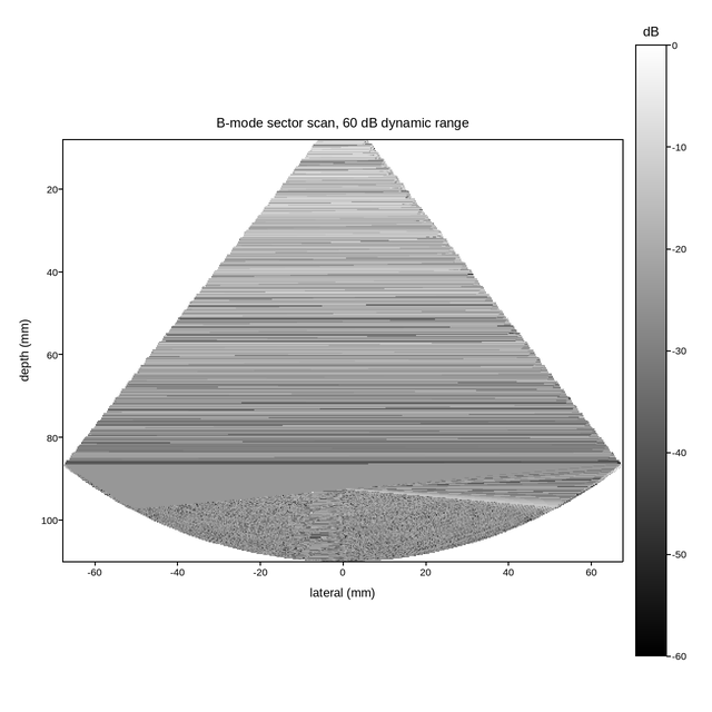
Live figure — pick a tool, then zoom, pan, point-pick or annotate. Nothing is active until a tool is selected.

View this figure’s Vega export ↗ — the raw JSON spec, rendered live by a real Vega engine.

View this figure’s Vega-Lite export ↗ — the raw JSON spec(s), rendered live by a real Vega-Lite engine.

import numpy as np
import polars as pl
import plotpress

rng = np.random.default_rng(31)
depth = np.linspace(10.0, 110.0, 340)                      # mm
angle = np.radians(np.linspace(-38.0, 38.0, 300))          # sector half-angle
D, A = np.meshgrid(depth, angle)
X = D * np.sin(A)
Y = D * np.cos(A)

# Rayleigh speckle is the baseline texture of soft tissue.
envelope = rng.rayleigh(1.0, D.shape)

# An anechoic cyst, a bright capsule, and attenuation with depth.
cyst = np.exp(-(((X - 14.0) ** 2 + (Y - 52.0) ** 2)) / 60.0)
envelope *= 1.0 - 0.93 * cyst
capsule = np.exp(-((np.hypot(X - 14.0, Y - 52.0) - 9.0) ** 2) / 1.2)
envelope += 7.0 * capsule
envelope += 5.0 * np.exp(-((Y - 88.0 - 0.18 * X) ** 2) / 3.0)   # fascial plane
envelope *= np.exp(-0.016 * D)                                   # 0.7 dB/cm/MHz

db = 20.0 * np.log10(envelope / envelope.max())
DYNAMIC_RANGE = 60.0
db = np.maximum(db, -DYNAMIC_RANGE)

# One row per (range, angle) beamformed sample -- the shape a scanner's own
# RF acquisition is in, before the curvilinear x/y mesh is reconstructed.
grid_shape = D.shape
frame = pl.DataFrame({
    "depth": D.ravel(), "angle": A.ravel(),
    "x": X.ravel(), "y": Y.ravel(), "db": db.ravel(),
}).sort(["depth", "angle"])
X = frame["x"].to_numpy().reshape(grid_shape)
Y = frame["y"].to_numpy().reshape(grid_shape)
db = frame["db"].to_numpy().reshape(grid_shape)

fig, ax = plotpress.subplots(figsize=(6.4, 6.4))
mesh = ax.pcolormesh(X, Y, db, cmap="gray", vmin=-DYNAMIC_RANGE, vmax=0.0)
fig.colorbar(mesh, ax=ax).set_title("dB")
ax.set_aspect("equal")
ax.invert_yaxis()
ax.set_xlabel("lateral (mm)")
ax.set_ylabel("depth (mm)")
ax.set_title(f"B-mode sector scan, {DYNAMIC_RANGE:.0f} dB dynamic range")
fig.tight_layout()