CT sinogram and reconstruction

What a CT scanner actually records is a sinogram: attenuation along every ray, indexed by detector position and gantry angle. A point off the rotation axis traces a sinusoid through it – hence the name – and the image only exists after reconstruction.

Both panels are meshes, and they want different treatment. The sinogram is a measurement in the projection domain: line integrals of attenuation, positive by construction, so a sequential map is right. The reconstruction is in Hounsfield units, a scale defined against water at 0 HU with air at -1000 and bone above +400. Zero is therefore physically meaningful, and the map is diverging about it – soft tissue slightly above water reads warm, fat and lung below it read cool.

Radiologists narrow the displayed range further still, to a window around the tissue of interest, which is exactly setting vmin/vmax rather than autoscaling. The soft-tissue window used here is the standard one.

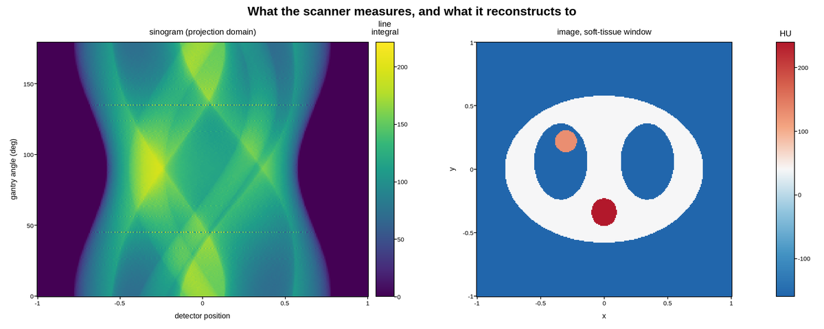
Live figure — pick a tool, then zoom, pan, point-pick or annotate. Nothing is active until a tool is selected.

View this figure’s Vega export ↗ — the raw JSON spec, rendered live by a real Vega engine.

View this figure’s Vega-Lite export ↗ — the raw JSON spec(s), rendered live by a real Vega-Lite engine.

import numpy as np
import polars as pl
import plotpress

N = 256
g = np.linspace(-1.0, 1.0, N)
X, Y = np.meshgrid(g, g)

# A phantom in Hounsfield units: body, lungs, spine, a lesion.
phantom = np.full_like(X, -1000.0)                       # air
body = (X ** 2 / 0.78 ** 2 + Y ** 2 / 0.58 ** 2) < 1.0
phantom[body] = 40.0                                      # soft tissue
for cx, cy in [(-0.34, 0.06), (0.34, 0.06)]:
    phantom[((X - cx) ** 2 / 0.21 ** 2 + (Y - cy) ** 2 / 0.30 ** 2) < 1.0] = -780.0
phantom[((X) ** 2 / 0.10 ** 2 + (Y + 0.34) ** 2 / 0.11 ** 2) < 1.0] = 620.0   # spine
phantom[((X + 0.30) ** 2 + (Y - 0.22) ** 2) < 0.0075] = 130.0                 # lesion

# Forward project: rotate the phantom and sum down columns.
angles = np.linspace(0.0, 180.0, 240, endpoint=False)
mu = (phantom + 1000.0) / 1000.0                          # attenuation, >= 0
sinogram = np.zeros((angles.size, N))
yy, xx = np.mgrid[0:N, 0:N]
cx = cy = (N - 1) / 2.0
for k, theta in enumerate(np.radians(angles)):
    xr = (xx - cx) * np.cos(theta) + (yy - cy) * np.sin(theta) + cx
    src = np.clip(np.rint(xr).astype(int), 0, N - 1)
    rotated = np.zeros((N, N))
    np.add.at(rotated, (yy, src), mu[yy, xx])
    sinogram[k] = rotated.sum(axis=0)

detector = np.linspace(-1.0, 1.0, N)
ANGLE, DETECTOR = np.meshgrid(angles, detector, indexing="ij")

# One row per detector reading -- the shape a CT gantry's own raw projection
# export is in, before it is gridded for the sinogram mesh.
projections = pl.DataFrame({
    "angle": ANGLE.ravel(), "detector": DETECTOR.ravel(), "line_integral": sinogram.ravel(),
}).sort(["angle", "detector"])
angles = projections["angle"].unique().sort().to_numpy()
detector = projections["detector"].unique().sort().to_numpy()
sinogram = projections["line_integral"].to_numpy().reshape(angles.size, detector.size)

# One row per reconstructed voxel -- the image-domain counterpart, gridded
# the same way once the reconstruction has been applied.
image = pl.DataFrame({"x": X.ravel(), "y": Y.ravel(), "hu": phantom.ravel()}) \
    .sort(["y", "x"])
g = image["x"].unique().sort().to_numpy()
phantom = image["hu"].to_numpy().reshape(g.size, g.size)

fig, axes = plotpress.subplots(1, 2, figsize=(12.0, 4.8))
sino = axes[0].pcolormesh(detector, angles, sinogram, cmap="viridis")
axes[0].set_title("sinogram (projection domain)")
axes[0].set_xlabel("detector position")
axes[0].set_ylabel("gantry angle (deg)")
fig.colorbar(sino, ax=axes[0]).set_title("line\nintegral")

WINDOW_LEVEL, WINDOW_WIDTH = 40.0, 400.0                  # soft-tissue window
img = axes[1].pcolormesh(g, g, phantom, cmap="RdBu_r",
                         vmin=WINDOW_LEVEL - WINDOW_WIDTH / 2,
                         vmax=WINDOW_LEVEL + WINDOW_WIDTH / 2)
axes[1].set_title("image, soft-tissue window")
axes[1].set_aspect("equal")
axes[1].set_xlabel("x")
axes[1].set_ylabel("y")
fig.colorbar(img, ax=axes[1]).set_title("HU")

fig.suptitle("What the scanner measures, and what it reconstructs to")
fig.tight_layout()