MRI k-space (LogNorm)

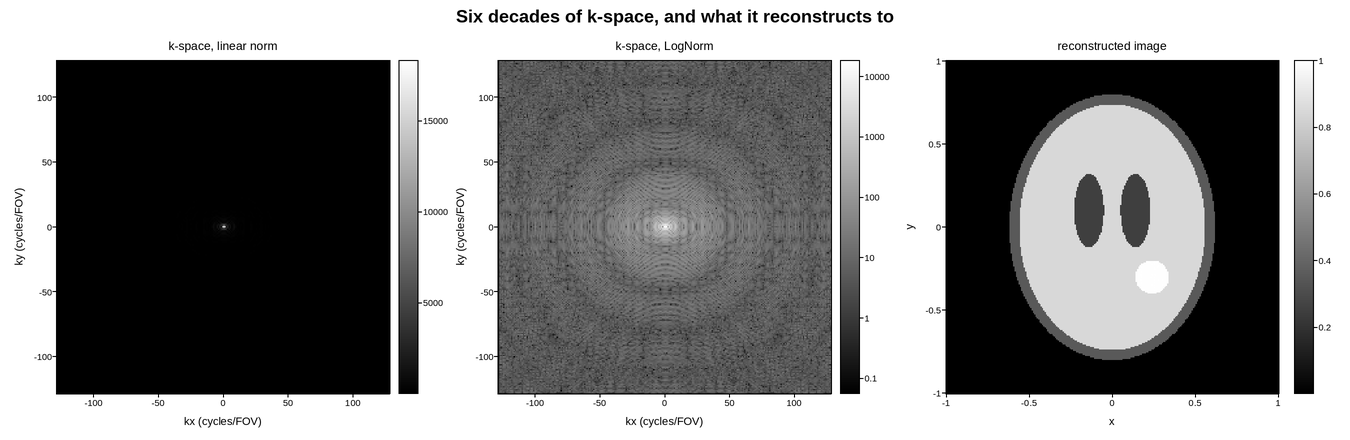
Raw MRI data is not an image. The scanner samples the Fourier transform of the slice – k-space – and the image only appears after an inverse transform. Radiographers inspect k-space directly because artefacts are legible there: spikes from gradient arcing, missing lines from a dropped trigger, motion as ghosting along the phase-encode direction.

Its dynamic range is extreme. The centre of k-space carries the bulk contrast and is four or five orders of magnitude above the edges, which carry the fine detail. Linearly normalised it is a single bright pixel on black. LogNorm makes the whole plane readable, which is the only way the sampling pattern and any dropout can be seen.

Shown beside the reconstructed image, so the correspondence is concrete.

Live figure — pick a tool, then zoom, pan, point-pick or annotate. Nothing is active until a tool is selected.

View this figure’s Vega export ↗ — the raw JSON spec, rendered live by a real Vega engine.

View this figure’s Vega-Lite export ↗ — the raw JSON spec(s), rendered live by a real Vega-Lite engine.

import numpy as np
import polars as pl
import plotpress

rng = np.random.default_rng(23)
N = 256
g = np.linspace(-1.0, 1.0, N)
X, Y = np.meshgrid(g, g)

# A crude head phantom: skull, brain, two ventricles, a lesion.
phantom = np.zeros_like(X)
phantom[(X ** 2 / 0.62 ** 2 + Y ** 2 / 0.80 ** 2) < 1.0] = 0.35      # skull
phantom[(X ** 2 / 0.56 ** 2 + Y ** 2 / 0.74 ** 2) < 1.0] = 0.85      # brain
for cx, cy, rx, ry in [(-0.14, 0.10, 0.09, 0.22), (0.14, 0.10, 0.09, 0.22)]:
    phantom[((X - cx) ** 2 / rx ** 2 + (Y - cy) ** 2 / ry ** 2) < 1.0] = 0.25
phantom[((X - 0.24) ** 2 + (Y + 0.30) ** 2) < 0.010] = 1.0           # lesion

kspace = np.fft.fftshift(np.fft.fft2(phantom))
magnitude = np.abs(kspace)
magnitude = np.maximum(magnitude, magnitude.max() * 1e-6)
kx = np.linspace(-N / 2, N / 2, N)
KX, KY = np.meshgrid(kx, kx)
X, Y = np.meshgrid(g, g)
reconstructed = np.abs(np.fft.ifft2(np.fft.ifftshift(kspace)))

# One row per k-space sample -- the shape a scanner's own raw data export is
# in, before it is gridded for the mesh.
acquisition = pl.DataFrame({"kx": KX.ravel(), "ky": KY.ravel(), "magnitude": magnitude.ravel()}) \
    .sort(["ky", "kx"])
kx = acquisition["kx"].unique().sort().to_numpy()
magnitude = acquisition["magnitude"].to_numpy().reshape(kx.size, kx.size)

# One row per reconstructed pixel -- the image-space counterpart, gridded
# the same way once the inverse transform has been applied.
image = pl.DataFrame({"x": X.ravel(), "y": Y.ravel(), "intensity": reconstructed.ravel()}) \
    .sort(["y", "x"])
g = image["x"].unique().sort().to_numpy()
reconstructed = image["intensity"].to_numpy().reshape(g.size, g.size)

fig, axes = plotpress.subplots(1, 3, figsize=(13.5, 4.4))
lin = axes[0].pcolormesh(kx, kx, magnitude, cmap="gray")
axes[0].set_title("k-space, linear norm")
fig.colorbar(lin, ax=axes[0])

log = axes[1].pcolormesh(kx, kx, magnitude, cmap="gray", norm=plotpress.LogNorm())
axes[1].set_title("k-space, LogNorm")
fig.colorbar(log, ax=axes[1])

img = axes[2].pcolormesh(g, g, reconstructed, cmap="gray")
axes[2].set_title("reconstructed image")
fig.colorbar(img, ax=axes[2])

for ax in axes[:2]:
    ax.set_xlabel("kx (cycles/FOV)")
    ax.set_ylabel("ky (cycles/FOV)")
axes[2].set_xlabel("x")
axes[2].set_ylabel("y")
for ax in axes:
    ax.set_aspect("equal")
fig.suptitle("Six decades of k-space, and what it reconstructs to")
fig.tight_layout()