Grain size distribution: which mean is the right mean

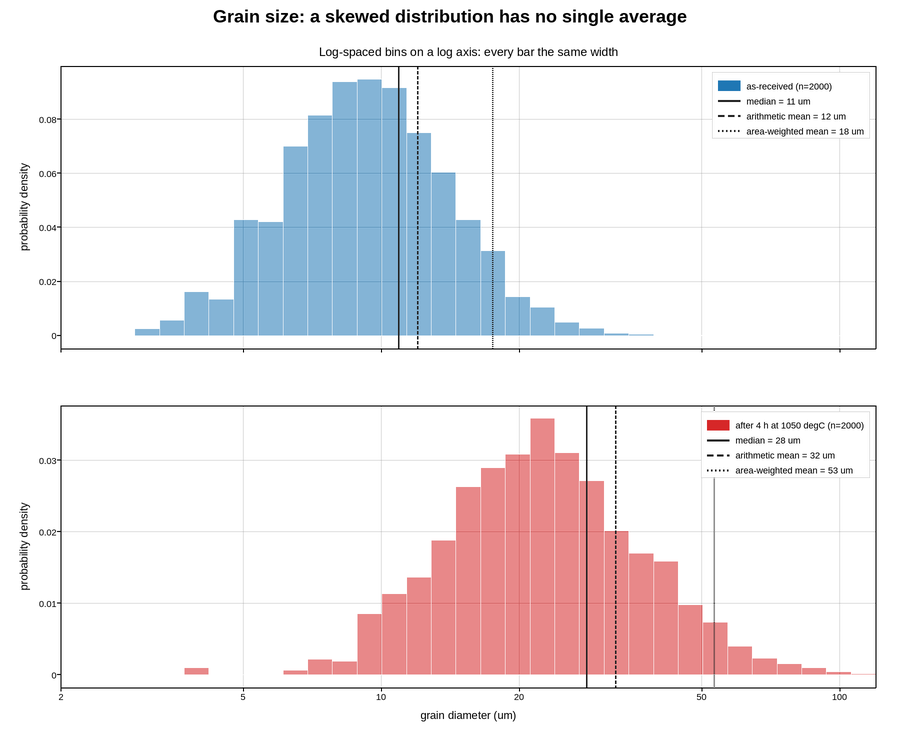
Two thousand grains measured from a micrograph, before and after a heat treatment. Grain size distributions are log-normal – growth is multiplicative, so the logarithm of the diameter is what is symmetric – and that single fact determines almost everything about the figure.

The histogram is plotted on a logarithmic x axis with logarithmically spaced bins. Equal-width bins on a log axis are the usual mistake: they render as progressively narrower bars toward the right and misrepresent the density, since a histogram bar’s area is the count. Bins spaced as logspace keep every bar the same width on screen, which is what makes the distribution look log-normal rather than merely skewed.

The other point is that a skewed distribution has no single “average grain size”. The arithmetic mean, the median and the area-weighted mean differ by nearly a factor of two here, and materials properties depend on different ones: yield strength follows the median through Hall-Petch, while thermal and optical behaviour follow the area-weighted value. All three are marked rather than one being quoted as “the” mean, and the anneal moves them by different amounts – which is the actual result of the experiment.

density=True rather than raw counts, so the two panels are comparable even though log-spaced bins have unequal widths in the underlying variable; a count histogram over unequal bins compares bar heights that mean different things.

Live figure — pick a tool, then zoom, pan, point-pick or annotate. Nothing is active until a tool is selected.

View this figure’s Vega export ↗ — the raw JSON spec, rendered live by a real Vega engine.

View this figure’s Vega-Lite export ↗ — the raw JSON spec(s), rendered live by a real Vega-Lite engine.

import numpy as np
import polars as pl
import plotpress

rng = np.random.default_rng(88)

N = 2000
BEFORE = (2.4, 0.42)                               # (log-mean, log-sigma), um
AFTER = (3.35, 0.50)                               # coarsened by annealing

bins = np.logspace(np.log10(2.0), np.log10(120.0), 34)

fig, axes = plotpress.subplots(2, 1, figsize=(9.0, 7.4), sharex=True)

for ax, (mu, sigma), label, color in [
        (axes[0], BEFORE, "as-received", "#1f77b4"),
        (axes[1], AFTER, "after 4 h at 1050 degC", "#d62728")]:
    # One row per measured grain -- the shape a micrograph's own grain-sizing
    # output is in, before the three competing means are computed from it.
    grains = pl.DataFrame({"diameter": rng.lognormal(mu, sigma, N)})
    d = grains["diameter"].to_numpy()

    ax.hist(d, bins=bins, color=color, alpha=0.55, edgecolor="#ffffff",
            density=True, label=f"{label} (n={N})")

    arithmetic = grains["diameter"].mean()
    median = grains["diameter"].median()
    # Area-weighted: each grain counts in proportion to its cross-section.
    area_weighted = float((grains["diameter"] ** 3).sum() / (grains["diameter"] ** 2).sum())

    for value, name, style in [(median, "median", "-"),
                               (arithmetic, "arithmetic mean", "--"),
                               (area_weighted, "area-weighted mean", ":")]:
        ax.axvline(value, color="#222222", linestyle=style, linewidth=1.4,
                   label=f"{name} = {value:.0f} um")

    ax.set_xscale("log")
    ax.set_ylabel("probability density")
    ax.legend(loc="upper right")
    ax.grid(True)

axes[0].set_title("Log-spaced bins on a log axis: every bar the same width")
axes[1].set_xlabel("grain diameter (um)")
axes[1].set_xlim(2.0, 120.0)

fig.suptitle("Grain size: a skewed distribution has no single average")
fig.tight_layout()