Tensile test: engineering and true stress

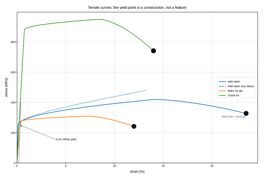
Stress against strain for three alloys pulled to failure, the measurement every structural property is quoted from. The figure carries two things a raw data plot would not: the construction that defines the yield strength, and the distinction between engineering and true stress.

Yield strength has no feature in the data to point at – the transition from elastic to plastic is gradual, so the definition is a convention: offset the elastic line by 0.2% strain and take the intersection. That construction line is drawn, because a number extracted by a convention should show the convention.

Engineering stress divides by the original cross-section, so once the specimen necks it reports a falling stress even though the material is still hardening. True stress divides by the instantaneous area and keeps rising. Plotting both for one alloy, as a solid and a dashed curve, is the compact way to show that the drop after the ultimate strength is a bookkeeping artefact rather than the material getting weaker.

Failure is a real endpoint, not a line running off the axis, so each curve stops at fracture and is marked there. Ductility – how far right the curve reaches – is as much a design property as the stress it reached.

Live figure — pick a tool, then zoom, pan, point-pick or annotate. Nothing is active until a tool is selected.

View this figure’s Vega export ↗ — the raw JSON spec, rendered live by a real Vega engine.

View this figure’s Vega-Lite export ↗ — the raw JSON spec(s), rendered live by a real Vega-Lite engine.

import numpy as np
import polars as pl
import plotpress

ALLOYS = [
    # name,        E (GPa), yield (MPa), UTS (MPa), fracture strain, colour
    ("mild steel",     205, 250, 420, 0.235, "#1f77b4"),
    ("6061-T6 alu",     69, 275, 310, 0.120, "#ff7f0e"),
    ("Ti-6Al-4V",      114, 880, 950, 0.140, "#2ca02c"),
]
OFFSET = 0.002                                     # 0.2% proof strain


def curve(E_gpa, yield_mpa, uts_mpa, eps_f, n=600):
    """Linear elastic to yield, then Hollomon power-law hardening to the UTS."""
    eps = np.linspace(0.0, eps_f, n)
    E = E_gpa * 1e3                                # MPa
    eps_y = yield_mpa / E
    plastic = np.clip(eps - eps_y, 0.0, None)
    eps_u = 0.6 * eps_f                            # strain at ultimate strength
    hardening = uts_mpa - yield_mpa
    sigma = yield_mpa + hardening * np.clip(plastic / (eps_u - eps_y), 0, 1) ** 0.5
    sigma = np.where(eps < eps_y, E * eps, sigma)
    # Necking: engineering stress falls after the ultimate point.
    neck = np.clip((eps - eps_u) / (eps_f - eps_u), 0.0, 1.0)
    return eps, sigma * (1.0 - 0.22 * neck ** 1.6)


# One row per strain-gauge sample -- the shape a tensile test's own
# extensometer log is in, before the yield construction is drawn over it.
runs = []
for name, E, sy, uts, eps_f, _ in ALLOYS:
    eps, sigma = curve(E, sy, uts, eps_f)
    runs.append(pl.DataFrame({"alloy": name, "strain": eps, "stress": sigma}))
tests = pl.concat(runs)

fig, ax = plotpress.subplots(figsize=(8.6, 5.8))

for name, E, sy, uts, eps_f, color in ALLOYS:
    run = tests.filter(pl.col("alloy") == name)
    eps = run["strain"].to_numpy()
    sigma = run["stress"].to_numpy()
    ax.plot(eps * 1e2, sigma, color=color, linewidth=1.9, label=name)
    ax.scatter([eps[-1] * 1e2], [sigma[-1]], s=11.0, color="#111111")

    if name == "mild steel":
        # True stress and strain, valid up to the onset of necking.
        upto = eps < 0.6 * eps_f
        ax.plot(np.log1p(eps[upto]) * 1e2, sigma[upto] * (1.0 + eps[upto]),
                color=color, linestyle="--", linewidth=1.4,
                label="mild steel, true stress")
        # The 0.2% offset construction that defines the yield strength.
        line_eps = np.array([OFFSET, OFFSET + sy / (E * 1e3) * 1.6])
        ax.plot(line_eps * 1e2, (line_eps - OFFSET) * E * 1e3,
                color="#333333", linestyle=":", linewidth=1.3)
        ax.annotate("0.2% offset yield", xy=(sy / (E * 1e3) * 1e2 + 0.2, sy),
                    xytext=(4.0, 150.0), arrowprops={"color": "#333333"},
                    fontsize=9)

ax.text(21.0, 300.0, "black dot = fracture", fontsize=9, color="#666666")
ax.set_xlim(0.0, None)
ax.set_ylim(0.0, None)
ax.set_xlabel("strain (%)")
ax.set_ylabel("stress (MPa)")
ax.set_title("Tensile curves: the yield point is a construction, not a feature")
ax.legend(loc="center right")
ax.grid(True)
fig.tight_layout()