XRD pole figure (curvilinear)

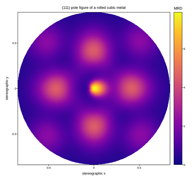
A pole figure from X-ray texture analysis: the sample is tilted and rotated while one reflection is monitored, so the measured intensity is a function of tilt and azimuth. That is a polar grid by construction, and projecting it stereographically gives 2-D X/Y node arrays – a genuinely curvilinear mesh rather than a rectangular image dressed up as one.

Intensity is quoted in multiples of a random distribution: 1.0 MRD is exactly what an untextured powder gives, and higher values mean grains preferentially aligned that way. So 1.0 is a meaningful reference but not a midpoint in the diverging sense – texture strength runs upward from it and is bounded below by zero, which makes a sequential map with the bar anchored at zero the honest choice.

The pattern here is a rolled cubic metal: a strong cube component at the centre with satellites near 45 degrees of tilt.

Live figure — pick a tool, then zoom, pan, point-pick or annotate. Nothing is active until a tool is selected.

View this figure’s Vega export ↗ — the raw JSON spec, rendered live by a real Vega engine.

View this figure’s Vega-Lite export ↗ — the raw JSON spec(s), rendered live by a real Vega-Lite engine.

import numpy as np
import polars as pl
import plotpress

tilt = np.radians(np.linspace(0.0, 80.0, 200))          # chi, from the pole
azimuth = np.radians(np.linspace(0.0, 360.0, 361))      # phi
CHI, PHI = np.meshgrid(tilt, azimuth, indexing="ij")

# Stereographic projection of the pole onto the equatorial plane.
radius = np.tan(CHI / 2.0)
X = radius * np.cos(PHI)
Y = radius * np.sin(PHI)

mrd = np.full_like(CHI, 0.35)


def component(chi0, phi0, spread, strength):
    """One texture component: a spot on the sphere, wrapped in azimuth."""
    dphi = np.angle(np.exp(1j * (PHI - phi0)))
    return strength * np.exp(-((CHI - chi0) ** 2 + (dphi * np.sin(CHI)) ** 2)
                             / (2 * spread ** 2))


mrd += component(0.0, 0.0, np.radians(11.0), 7.5)                 # cube
for k in range(4):                                                 # satellites
    mrd += component(np.radians(45.0), k * np.pi / 2, np.radians(13.0), 4.2)
for k in range(4):
    mrd += component(np.radians(72.0), np.pi / 4 + k * np.pi / 2,
                     np.radians(10.0), 1.9)

# One row per (chi, phi) goniometer step -- the shape a texture goniometer's
# own scan log is in, before the curvilinear x/y mesh is reconstructed.
grid_shape = CHI.shape
scan = pl.DataFrame({
    "chi": CHI.ravel(), "phi": PHI.ravel(),
    "x": X.ravel(), "y": Y.ravel(), "mrd": mrd.ravel(),
}).sort(["chi", "phi"])
X = scan["x"].to_numpy().reshape(grid_shape)
Y = scan["y"].to_numpy().reshape(grid_shape)
mrd = scan["mrd"].to_numpy().reshape(grid_shape)

fig, ax = plotpress.subplots(figsize=(6.2, 5.8))
mesh = ax.pcolormesh(X, Y, mrd, cmap="plasma", vmin=0.0)
fig.colorbar(mesh, ax=ax).set_title("MRD")
ax.set_aspect("equal")
ax.set_xlabel("stereographic x")
ax.set_ylabel("stereographic y")
ax.set_title("(111) pole figure of a rolled cubic metal")
fig.tight_layout()