Boundary-layer profiles in wall units

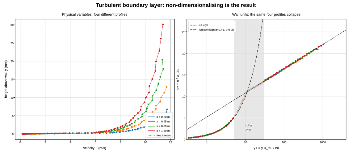
Velocity profiles measured at four positions along a flat plate, plotted twice. The left panel uses the physical variables – height above the wall, velocity – and shows four different curves that grow thicker downstream. The right panel uses wall units, and the same four measurements collapse onto one curve.

That collapse is the result. Non-dimensionalising by the friction velocity and the viscous length scale is what turns four datasets into one universal profile, and the only way to show it is to plot both forms side by side. A figure showing only the collapsed version would be a claim; showing both is the evidence.

The right panel is semi-logarithmic in the wall-normal coordinate because the structure being tested is logarithmic: the log law appears as a straight line over the region where it applies, and its slope and intercept are the constants being checked. On a linear axis the viscous sublayer – three decades below the outer edge – would be invisible, and the log region would be an unremarkable curve.

The two analytic limits, u+ = y+ in the sublayer and the log law above it, are drawn as dashed lines so the reader can see where each stops describing the data, and the buffer layer between them is shaded because neither applies there.

Live figure — pick a tool, then zoom, pan, point-pick or annotate. Nothing is active until a tool is selected.

View this figure’s Vega export ↗ — the raw JSON spec, rendered live by a real Vega engine.

View this figure’s Vega-Lite export ↗ — the raw JSON spec(s), rendered live by a real Vega-Lite engine.

import numpy as np
import polars as pl
import plotpress

rng = np.random.default_rng(1904)

KAPPA, B = 0.41, 5.2                               # von Karman constant, intercept
NU = 1.5e-5                                        # kinematic viscosity, m2/s
U_INF = 12.0                                       # free-stream velocity, m/s

STATIONS = [(0.20, "#1f77b4"), (0.45, "#ff7f0e"),
            (0.80, "#2ca02c"), (1.30, "#d62728")]


def u_plus(y_plus):
    """Spalding-style blend of the viscous sublayer and the log law."""
    log_law = np.log(np.maximum(y_plus, 1e-6)) / KAPPA + B
    blend = np.exp(-(y_plus / 11.0) ** 4)
    return blend * y_plus + (1.0 - blend) * log_law


station_profiles = []
for x_station, _ in STATIONS:
    # Turbulent flat-plate correlations: skin friction falls slowly downstream.
    re_x = U_INF * x_station / NU
    cf = 0.0592 * re_x ** -0.2
    u_tau = U_INF * np.sqrt(cf / 2.0)
    delta = 0.37 * x_station * re_x ** -0.2        # boundary-layer thickness

    y_plus = np.logspace(np.log10(0.3), np.log10(u_tau * delta / NU), 60)
    y = y_plus * NU / u_tau
    u = np.minimum(u_plus(y_plus), U_INF / u_tau) * u_tau
    u = u * (1.0 + rng.normal(0.0, 0.006, u.size))  # hot-wire noise

    # One row per probe position -- the shape a hot-wire traverse's own
    # output is in, before the physical and wall-unit views are plotted.
    station_profiles.append(pl.DataFrame({
        "x_station": x_station, "y": y, "u": u, "y_plus": y_plus, "u_tau": u_tau,
    }))
profiles = pl.concat(station_profiles)

fig, axes = plotpress.subplots(1, 2, figsize=(11.4, 5.0))
ax_phys, ax_wall = axes

for x_station, color in STATIONS:
    probe = profiles.filter(pl.col("x_station") == x_station)
    y = probe["y"].to_numpy()
    u = probe["u"].to_numpy()
    y_plus = probe["y_plus"].to_numpy()
    u_tau = probe["u_tau"][0]

    # plot() draws the line and scatter() the sample markers: these are 60
    # discrete probe positions, not a continuous curve, and the marker spacing
    # is how a reader sees where the traverse actually sampled.
    ax_phys.plot(u, y * 1e3, color=color, linewidth=1.2,
                 label=f"x = {x_station:.2f} m")
    ax_phys.scatter(u, y * 1e3, s=3.5, color=color)
    ax_wall.scatter(y_plus, u / u_tau, s=3.5, color=color)

ax_phys.axvline(U_INF, color="#888888", linestyle=":", linewidth=1.2,
                label="free stream")
ax_phys.set_xlabel("velocity u (m/s)")
ax_phys.set_ylabel("height above wall y (mm)")
ax_phys.set_title("Physical variables: four different profiles")
ax_phys.legend(loc="lower right")
ax_phys.grid(True)

grid = np.logspace(np.log10(0.3), 3.6, 200)
ax_wall.axvspan(5.0, 30.0, color="#dddddd", alpha=0.7)
ax_wall.text(12.0, 3.0, "buffer\nlayer", ha="center", fontsize=9, color="#555555")
sublayer = grid[grid <= 30.0]          # the asymptote only claims this region
ax_wall.plot(sublayer, sublayer, color="#333333", linestyle="--", linewidth=1.3,
             label="u+ = y+")
ax_wall.plot(grid, np.log(grid) / KAPPA + B, color="#333333", linestyle="-.",
             linewidth=1.3, label=f"log law (kappa={KAPPA}, B={B})")
ax_wall.set_xscale("log")
ax_wall.set_xlim(0.3, 4000.0)
ax_wall.set_ylim(0.0, 28.0)
ax_wall.set_xlabel("y+ = y u_tau / nu")
ax_wall.set_ylabel("u+ = u / u_tau")
ax_wall.set_title("Wall units: the same four profiles collapse")
ax_wall.legend(loc="upper left")
ax_wall.grid(True)

fig.suptitle("Turbulent boundary layer: non-dimensionalising is the result")
fig.tight_layout()