Pump curve and system curve

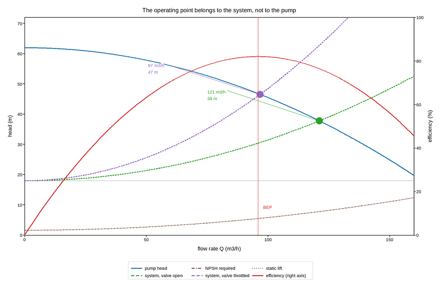
Where a centrifugal pump actually runs is not a property of the pump. It is the intersection of the pump’s head-flow curve with the system’s resistance curve, and the only way to see it is to draw both on the same axes – which is what this figure is for.

The pump curve falls with flow; the system curve rises as the square of it, because pipe friction is quadratic in velocity. They cross once, and that crossing is the operating point. Throttling a valve steepens the system curve and slides the point up and to the left, which is drawn here as a second system curve rather than described, because the movement of the intersection is the insight.

Efficiency lives on a different scale entirely – percent, not metres – so it goes on a twin axis. This is the honest use of twinx: the two quantities share the flow axis and genuinely nothing else, and the reader is being asked to compare their x positions, not their heights. The best-efficiency point is marked on both, because a pump running far from it is the single most common cause of premature seal and bearing failure, and the distance between the operating point and the BEP is the number this figure exists to produce.

NPSH required is drawn too, on the same head axis as the pump curve since both are in metres – a rare case where two curves legitimately share one axis despite meaning different things.

Live figure — pick a tool, then zoom, pan, point-pick or annotate. Nothing is active until a tool is selected.

View this figure’s Vega export ↗ — the raw JSON spec, rendered live by a real Vega engine.

View this figure’s Vega-Lite export ↗ — the raw JSON spec(s), rendered live by a real Vega-Lite engine.

import numpy as np
import polars as pl
import plotpress

flow = np.linspace(0.0, 160.0, 400)                # m3/h

SHUTOFF_HEAD = 62.0                                # m at zero flow
Q_BEP = 96.0                                       # best-efficiency flow

# One row per flow rate -- the shape a pump's own test-stand data sheet is in,
# before the operating point is picked out against a system curve.
pump = pl.DataFrame({
    "flow": flow,
    "head": SHUTOFF_HEAD - 0.00165 * flow ** 2,
    "efficiency": 82.0 * (1.0 - ((flow - Q_BEP) / 96.0) ** 2) * (flow > 0),
    "npsh_required": 1.6 + 0.00042 * flow ** 2,
})
flow = pump["flow"].to_numpy()
head_pump = pump["head"].to_numpy()
efficiency = pump["efficiency"].to_numpy()
npsh_required = pump["npsh_required"].to_numpy()

STATIC_LIFT = 18.0                                 # m the fluid must be raised
SYSTEMS = [("valve open", 0.00135, "#2ca02c"),
           ("valve throttled", 0.00305, "#9467bd")]

# One row per (system, flow rate) point -- the two resistance curves the
# pump curve is intersected against.
system_curves = pl.concat([
    pl.DataFrame({"system": name, "flow": flow, "head": STATIC_LIFT + k * flow ** 2})
    for name, k, _ in SYSTEMS
])

fig, ax = plotpress.subplots(figsize=(9.0, 5.8))
ax.plot(flow, head_pump, color="#1f77b4", linewidth=2.2, label="pump head")
ax.plot(flow, npsh_required, color="#8c564b", linewidth=1.5, linestyle="-.",
        label="NPSH required")
ax.axhline(STATIC_LIFT, color="#888888", linestyle=":", linewidth=1.2,
           label="static lift")

for name, k, color in SYSTEMS:
    head_system = system_curves.filter(pl.col("system") == name)["head"].to_numpy()
    ax.plot(flow, head_system, color=color, linewidth=1.8, linestyle="--",
            label=f"system, {name}")
    # Operating point: where the two curves cross.
    q_op = float(np.interp(0.0, head_system - head_pump, flow))
    h_op = float(np.interp(q_op, flow, head_pump))
    ax.scatter([q_op], [h_op], s=10.0, color=color)
    ax.annotate(f"{q_op:.0f} m3/h\n{h_op:.0f} m", xy=(q_op, h_op),
                xytext=(q_op - 46.0, h_op + 9.0), fontsize=9, color=color,
                arrowprops={"color": color})

ax.axvline(Q_BEP, color="#d62728", linestyle=":", linewidth=1.4)
ax.set_xlim(0.0, 160.0)
ax.set_ylim(0.0, 72.0)
ax.set_xlabel("flow rate Q (m3/h)")
ax.set_ylabel("head (m)")

ax2 = ax.twinx()
ax2.plot(flow, efficiency, color="#d62728", linewidth=1.6,
         label="efficiency (right axis)")
ax2.set_ylabel("efficiency (%)")
ax2.set_ylim(0.0, 100.0)
ax2.text(Q_BEP + 2.0, 12.0, "BEP", fontsize=9, color="#d62728")

ax.set_title("The operating point belongs to the system, not to the pump")
fig.legend(ax=[ax, ax2], loc="lower center", ncol=3)
fig.tight_layout()