Heat exchanger tube bundle

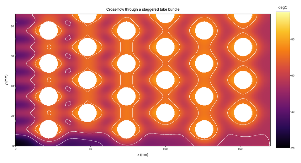
Fluid temperature through a staggered tube bundle in cross-flow, the core of a shell-and-tube heat exchanger. Cold fluid enters from the left and is heated as it passes rows of hot tubes; the staggered arrangement forces it to weave, which is what makes the bundle exchange heat efficiently.

Temperature has a physically meaningful floor and ceiling here – inlet and tube-wall temperature – and the reading of interest is where the fluid sits between them, so a sequential map spanning exactly that range is right, with the limits pinned rather than autoscaled. Fixing them means this figure can be compared directly against a run at a different flow rate.

The tubes themselves are solid metal, not fluid: they are nan, so they appear as holes in the field rather than as regions of some invented temperature. Isotherms over the mesh show the thermal boundary layers wrapping each tube.

Live figure — pick a tool, then zoom, pan, point-pick or annotate. Nothing is active until a tool is selected.

View this figure’s Vega export ↗ — the raw JSON spec, rendered live by a real Vega engine.

View this figure’s Vega-Lite export ↗ — the raw JSON spec(s), rendered live by a real Vega-Lite engine.

import numpy as np
import polars as pl
import plotpress

T_IN, T_WALL = 20.0, 95.0          # degC
TUBE_R = 6.0                       # mm
PITCH_X, PITCH_Y = 26.0, 22.0

x = np.linspace(0.0, 170.0, 380)   # mm
y = np.linspace(0.0, 88.0, 300)
X, Y = np.meshgrid(x, y)

# Staggered bundle: every other column offset by half a pitch.
centres = []
for i in range(6):
    cx = 22.0 + i * PITCH_X
    offset = 0.5 * PITCH_Y if i % 2 else 0.0
    for j in range(4):
        centres.append((cx, 11.0 + offset + j * PITCH_Y))

# Bulk fluid warms along the bundle; each tube adds a local thermal boundary
# layer that is swept downstream of it.
temperature = T_IN + (T_WALL - T_IN) * 0.55 * (1.0 - np.exp(-X / 90.0))
for cx, cy in centres:
    r = np.hypot(X - cx, Y - cy)
    near = np.exp(-((r - TUBE_R) ** 2) / 34.0)
    wake = np.exp(-((Y - cy) ** 2) / 26.0) * np.exp(-np.clip(X - cx, 0.0, None) / 14.0)
    temperature += (T_WALL - temperature) * (0.42 * near + 0.16 * wake)

for cx, cy in centres:             # the tubes carry no fluid temperature
    temperature[np.hypot(X - cx, Y - cy) < TUBE_R] = np.nan

# One row per grid node -- the shape a CFD solver's own field export is in,
# before it is gridded for the mesh and contour. The tubes' nan cells ride
# along in the value column; the x/y axis columns stay finite throughout.
field = pl.DataFrame({"x": X.ravel(), "y": Y.ravel(), "temperature": temperature.ravel()}) \
    .sort(["y", "x"])
x = field["x"].unique().sort().to_numpy()
y = field["y"].unique().sort().to_numpy()
temperature = field["temperature"].to_numpy().reshape(y.size, x.size)
X, Y = np.meshgrid(x, y)

fig, ax = plotpress.subplots(figsize=(9.6, 5.2))
mesh = ax.pcolormesh(x, y, temperature, cmap="inferno", vmin=T_IN, vmax=T_WALL)
ax.contour(X, Y, np.nan_to_num(temperature, nan=T_WALL),
           levels=[40.0, 55.0, 70.0, 85.0], colors="#ffffff")
fig.colorbar(mesh, ax=ax).set_title("degC")
ax.set_aspect("equal")
ax.set_xlabel("x (mm)")
ax.set_ylabel("y (mm)")
ax.set_title("Cross-flow through a staggered tube bundle")
fig.tight_layout()