Steady-state conduction, with isotherms

Temperature in a rectangular plate held at 0 degC on three edges and 100 degC along the top – the classical Fourier-series solution of Laplace’s equation.

The field is the mesh; the isotherms are contour drawn straight over it. Pass contour the same 2-D X/Y you gave pcolormesh and the two line up exactly, which is the usual way to read a magnitude and its level sets at once.

The series is truncated at 40 terms, so it overshoots by roughly 15% in the two top corners where the boundary condition jumps from 0 to 100 – ordinary Gibbs ringing, not a plotting artifact. The color limits are pinned to the physical range so the overshoot saturates instead of stretching the scale past 100.

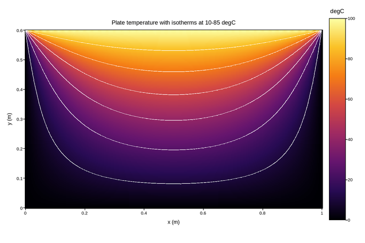
Live figure — pick a tool, then zoom, pan, point-pick or annotate. Nothing is active until a tool is selected.

View this figure’s Vega export ↗ — the raw JSON spec, rendered live by a real Vega engine.

View this figure’s Vega-Lite export ↗ — the raw JSON spec(s), rendered live by a real Vega-Lite engine.

import numpy as np
import polars as pl
import plotpress

L, W = 1.0, 0.6          # plate width and height (m)
T_TOP = 100.0            # temperature of the top edge (degC)

x = np.linspace(0.0, L, 260)
y = np.linspace(0.0, W, 170)
X, Y = np.meshgrid(x, y)

# T(x, y) = sum over odd n of (4 T / n pi) sin(n pi x / L) sinh(n pi y / L)
#                                          / sinh(n pi W / L)
# The sinh ratio is written as an exponential difference so the large-n terms
# stay finite instead of dividing two enormous numbers.
T = np.zeros_like(X)
for n in range(1, 80, 2):        # 40 odd harmonics
    k = n * np.pi / L
    ratio = (np.exp(k * (Y - W)) - np.exp(-k * (Y + W))) / (1.0 - np.exp(-2.0 * k * W))
    T += (4.0 * T_TOP / (n * np.pi)) * np.sin(k * X) * ratio

# One row per grid node -- the shape a finite-element solver's own field
# export is in, before it is gridded for the mesh and contour.
field = pl.DataFrame({"x": X.ravel(), "y": Y.ravel(), "temperature": T.ravel()}) \
    .sort(["y", "x"])
x = field["x"].unique().sort().to_numpy()
y = field["y"].unique().sort().to_numpy()
T = field["temperature"].to_numpy().reshape(y.size, x.size)
X, Y = np.meshgrid(x, y)

fig, ax = plotpress.subplots(figsize=(7.5, 5))
mesh = ax.pcolormesh(x, y, T, cmap="inferno", vmin=0.0, vmax=T_TOP)
ax.contour(X, Y, T, levels=[10.0, 25.0, 40.0, 55.0, 70.0, 85.0], colors="white")
bar = fig.colorbar(mesh, ax=ax)
bar.set_title("degC")
ax.set_aspect("equal")
ax.set_xlabel("x (m)")
ax.set_ylabel("y (m)")
ax.set_title("Plate temperature with isotherms at 10-85 degC")
fig.tight_layout()