Efficient frontier from random portfolios

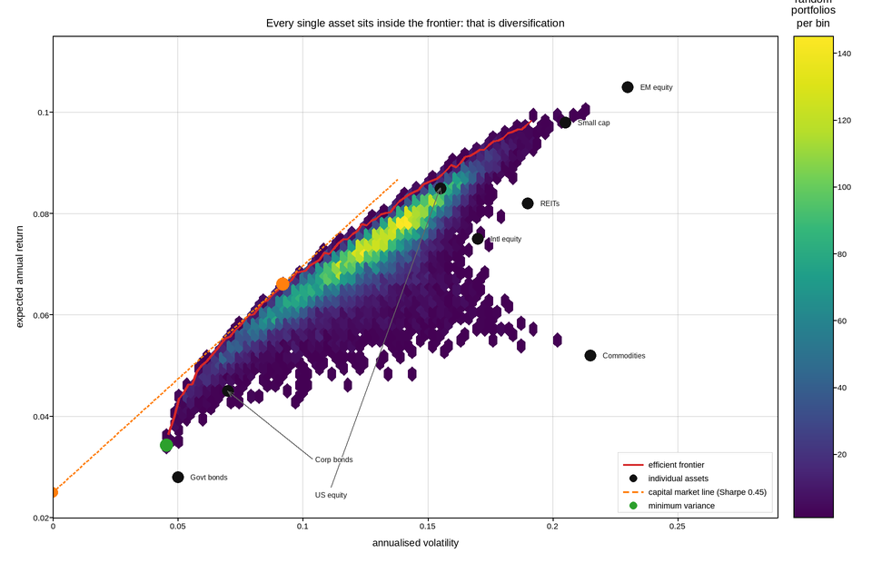
Twenty thousand randomly weighted portfolios of eight assets, plotted as expected return against volatility, with the efficient frontier traced along their upper-left edge. The cloud is the point: the frontier is not a curve somebody drew, it is the boundary of what is achievable, and showing the achievable set is what makes that credible.

Twenty thousand points need binning rather than markers, so the cloud is a hexbin. Its density is worth reading in its own right: random weightings pile up in the middle of the achievable set and thin out toward the frontier, which is a direct statement that good portfolios are rare and are not found by accident.

The frontier itself is computed by taking the maximum return within each volatility bin, which is the definition, and drawn as a line. The individual assets are marked, and the fact that every one of them lies inside the frontier is the case for diversification stated as geometry.

The capital market line – the tangent from the risk-free rate – is drawn because the tangency portfolio, not the minimum-variance portfolio, is the one an investor who can borrow and lend should hold. Both are marked, since the distinction is the most commonly skipped step in reading this figure.

Live figure — pick a tool, then zoom, pan, point-pick or annotate. Nothing is active until a tool is selected.

View this figure’s Vega export ↗ — the raw JSON spec, rendered live by a real Vega engine.

View this figure’s Vega-Lite export ↗ — the raw JSON spec(s), rendered live by a real Vega-Lite engine.

import numpy as np
import polars as pl
import plotpress

rng = np.random.default_rng(1952)

ASSETS = ["US equity", "Intl equity", "EM equity", "Small cap",
          "Corp bonds", "Govt bonds", "REITs", "Commodities"]

# One row per asset -- the shape a fund's own return/risk assumptions sheet
# is in, before it is turned into a covariance matrix.
asset_stats = pl.DataFrame({
    "asset": ASSETS,
    "mean_return": [0.085, 0.075, 0.105, 0.098, 0.045, 0.028, 0.082, 0.052],
    "volatility": [0.155, 0.170, 0.230, 0.205, 0.070, 0.050, 0.190, 0.215],
})
mean_return = asset_stats["mean_return"].to_numpy()
volatility = asset_stats["volatility"].to_numpy()
RISK_FREE = 0.025

# A plausible correlation structure: equities move together, bonds hedge them.
corr = np.array([
    [1.00, 0.85, 0.72, 0.90, 0.20, -0.15, 0.65, 0.30],
    [0.85, 1.00, 0.78, 0.80, 0.18, -0.12, 0.60, 0.32],
    [0.72, 0.78, 1.00, 0.70, 0.15, -0.10, 0.55, 0.40],
    [0.90, 0.80, 0.70, 1.00, 0.18, -0.14, 0.68, 0.28],
    [0.20, 0.18, 0.15, 0.18, 1.00, 0.62, 0.30, 0.05],
    [-0.15, -0.12, -0.10, -0.14, 0.62, 1.00, 0.05, -0.08],
    [0.65, 0.60, 0.55, 0.68, 0.30, 0.05, 1.00, 0.25],
    [0.30, 0.32, 0.40, 0.28, 0.05, -0.08, 0.25, 1.00],
])
cov = corr * np.outer(volatility, volatility)

N = 20000
weights = rng.dirichlet(np.full(len(ASSETS), 0.7), N)

# One row per randomly weighted portfolio -- the shape a Monte Carlo sweep's
# own output table is in, before the frontier is picked out of the cloud.
portfolios = pl.DataFrame({
    "volatility": np.sqrt(np.einsum("ij,jk,ik->i", weights, cov, weights)),
    "return": weights @ mean_return,
})
portfolios = portfolios.with_columns(
    ((pl.col("return") - RISK_FREE) / pl.col("volatility")).alias("sharpe"))
port_vol = portfolios["volatility"].to_numpy()
port_return = portfolios["return"].to_numpy()
sharpe = portfolios["sharpe"].to_numpy()

fig, ax = plotpress.subplots(figsize=(9.6, 6.2))

hb = ax.hexbin(port_vol, port_return, gridsize=52, cmap="viridis", mincnt=1)
fig.colorbar(hb, ax=ax).set_title("random\nportfolios\nper bin")

# The frontier is the maximum return achieved in each volatility bin -- which
# is its definition, so it comes out of the cloud rather than being fitted to it.
bins = np.linspace(port_vol.min(), port_vol.max(), 90)
idx = np.clip(np.digitize(port_vol, bins) - 1, 0, bins.size - 2)
frontier_vol, frontier_ret = [], []
for b in range(bins.size - 1):
    sel = idx == b
    if sel.sum() >= 5:
        frontier_vol.append(port_vol[sel].mean())
        frontier_ret.append(port_return[sel].max())

ax.plot(frontier_vol, frontier_ret, color="#d62728", linewidth=2.4,
        label="efficient frontier")
ax.scatter(volatility, mean_return, s=9.0, color="#111111",
           label="individual assets")
# A marker sitting in the cloud cannot take a label beside it: the cloud runs
# from near-black to bright yellow, so no single ink is readable across it.
# Those get a leader out to clear space instead. Nudging the label a little way
# off is the worst of both -- still on the cloud, and now far enough from its
# marker that the reader has to guess which dot it belongs to.
crowded = np.array([((np.abs(port_vol - v) < 0.008)
                     & (np.abs(port_return - r) < 0.005)).sum() > 40
                    for v, r in zip(volatility, mean_return)])
# The strip below the cloud and left of the legend is the one reliably empty
# part of the panel, so every leader ends there, stacked.
led = 0
for k, (name, v, r) in enumerate(zip(ASSETS, volatility, mean_return)):
    if crowded[k]:
        ax.annotate(name, xy=(v, r), xytext=(0.105, 0.0245 + 0.007 * led),
                    fontsize=8, va="center", color="#111111",
                    arrowprops={"color": "#666666"})
        led += 1
    else:
        ax.text(v + 0.005, r, name, fontsize=8, va="center", color="#111111")

tangency = int(np.argmax(sharpe))
minvar = int(np.argmin(port_vol))
ax.plot([0.0, port_vol[tangency] * 1.5],
        [RISK_FREE, RISK_FREE + sharpe[tangency] * port_vol[tangency] * 1.5],
        color="#ff7f0e", linewidth=1.7, linestyle="--",
        label=f"capital market line (Sharpe {sharpe[tangency]:.2f})")
ax.scatter([port_vol[tangency]], [port_return[tangency]], s=10.0, color="#ff7f0e")
ax.scatter([port_vol[minvar]], [port_return[minvar]], s=10.0, color="#2ca02c",
           label="minimum variance")
ax.scatter([0.0], [RISK_FREE], s=8.0, color="#ff7f0e")

ax.set_xlim(0.0, 0.29)
ax.set_ylim(0.02, 0.115)
ax.set_xlabel("annualised volatility")
ax.set_ylabel("expected annual return")
ax.set_title("Every single asset sits inside the frontier: that is diversification")
ax.legend(loc="lower right")
ax.grid(True)
fig.tight_layout()