Yield curve evolution and the 2s10s spread

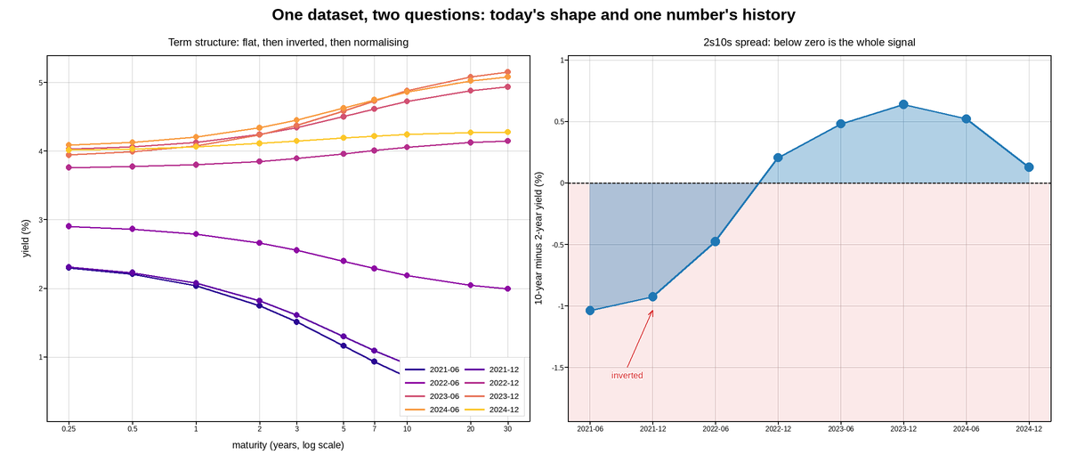
The term structure of interest rates at eight dates, and the spread between the two-year and ten-year points over the same period. The two panels answer different questions from one dataset: the shape of the curve on a given day, and the history of one number derived from it.

The maturity axis is logarithmic because the standard maturities are spaced 1, 2, 3, 5, 7, 10, 20, 30 years – geometric, not arithmetic. On a linear axis the short end, where central-bank policy is transmitted and where the curve does almost all of its moving, occupies a tenth of the width.

The eight curves are one continuous variable – time – so they are coloured by sampling a sequential colormap rather than the categorical cycle, and the legend runs in date order. This is the same reasoning as the transistor family elsewhere in the gallery: the reader should be able to see the direction of travel without matching eight unrelated hues to eight dates.

Inversion is the event these plots exist to catch: when the ten-year yield falls below the two-year, the curve slopes down and the spread goes negative. The negative region of the right panel is shaded, and it is the one place a signed quantity crossing zero justifies breaking the fill into two colours.

Live figure — pick a tool, then zoom, pan, point-pick or annotate. Nothing is active until a tool is selected.

View this figure’s Vega export ↗ — the raw JSON spec, rendered live by a real Vega engine.

View this figure’s Vega-Lite export ↗ — the raw JSON spec(s), rendered live by a real Vega-Lite engine.

import numpy as np
import polars as pl
import plotpress

MATURITIES = np.array([0.25, 0.5, 1, 2, 3, 5, 7, 10, 20, 30], float)

# (label, short-rate level, slope, curvature) -- a Nelson-Siegel style shape.
DATES = [
    ("2021-06", 0.10, 2.30, 0.55),
    ("2021-12", 0.35, 2.05, 0.50),
    ("2022-06", 1.90, 1.05, 0.30),
    ("2022-12", 4.20, -0.45, -0.20),
    ("2023-06", 5.05, -1.05, -0.45),
    ("2023-12", 5.30, -1.40, -0.55),
    ("2024-06", 5.20, -1.15, -0.40),
    ("2024-12", 4.30, -0.30, 0.05),
]
TAU = 2.2


def nelson_siegel(level, slope, curvature):
    x = MATURITIES / TAU
    decay = (1.0 - np.exp(-x)) / x
    return level + slope * decay + curvature * (decay - np.exp(-x))


lut = plotpress.get_cmap("plasma")
colors = ["#%02x%02x%02x" % tuple(lut[i])
          for i in np.linspace(15, 225, len(DATES)).astype(int)]

fig, axes = plotpress.subplots(1, 2, figsize=(12.0, 5.2))
ax_curve, ax_spread = axes

# One row per (date, maturity) point -- the shape a term-structure history is
# actually published in, before the 2s10s spread is computed from it.
curves = pl.concat([
    pl.DataFrame({"date": label, "maturity": MATURITIES,
                  "yield": nelson_siegel(level, slope, curvature)})
    for label, level, slope, curvature in DATES
])

spreads, positions = [], np.arange(len(DATES), dtype=float)
for (label, level, slope, curvature), color in zip(DATES, colors):
    date_curve = curves.filter(pl.col("date") == label)
    maturity = date_curve["maturity"].to_numpy()
    yields = date_curve["yield"].to_numpy()
    ax_curve.plot(maturity, yields, color=color, linewidth=1.8, label=label)
    ax_curve.scatter(maturity, yields, s=4.5, color=color)
    spreads.append(float(np.interp(10.0, maturity, yields)
                         - np.interp(2.0, maturity, yields)))

ax_curve.set_xscale("log")
ax_curve.set_xticks(MATURITIES, [f"{m:g}" for m in MATURITIES])
ax_curve.tick_params(labelsize=8)
ax_curve.set_xlabel("maturity (years, log scale)")
ax_curve.set_ylabel("yield (%)")
ax_curve.set_title("Term structure: flat, then inverted, then normalising")
ax_curve.legend(loc="lower right", ncol=2)
ax_curve.grid(True)

spreads = np.array(spreads)
ax_spread.axhspan(-2.0, 0.0, color="#d62728", alpha=0.10)
ax_spread.fill_between(positions, spreads, 0.0, color="#1f77b4", alpha=0.35)
ax_spread.plot(positions, spreads, color="#1f77b4", linewidth=2.0)
ax_spread.scatter(positions, spreads, s=7.0, color="#1f77b4")
ax_spread.axhline(0.0, color="#333333", linewidth=1.4)

inverted = positions[spreads < 0]
if inverted.size:
    ax_spread.annotate("inverted", xy=(inverted.mean(), spreads.min()),
                       xytext=(inverted.mean() - 0.4, spreads.min() - 0.55),
                       arrowprops={"color": "#d62728"}, color="#d62728",
                       fontsize=10, ha="center")

ax_spread.set_xticks(positions, [label for label, *_ in DATES])
ax_spread.tick_params(labelsize=8)
ax_spread.set_ylim(spreads.min() - 0.9, max(spreads.max() + 0.4, 0.5))
ax_spread.set_ylabel("10-year minus 2-year yield (%)")
ax_spread.set_title("2s10s spread: below zero is the whole signal")
ax_spread.grid(True)

fig.suptitle("One dataset, two questions: today's shape and one number's history")
fig.tight_layout()