Photovoltaic I-V and power curves

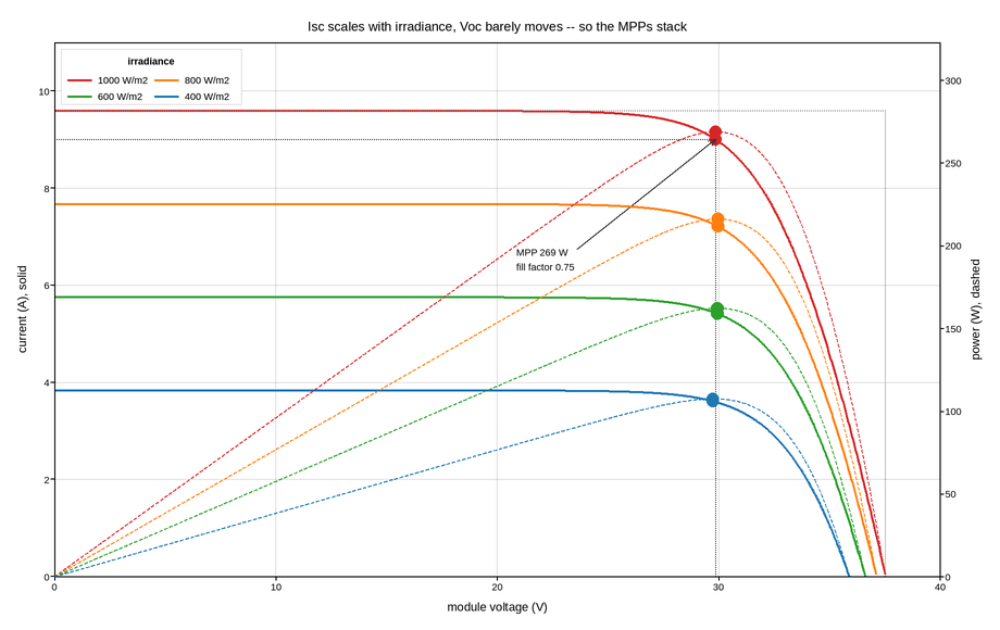
A solar module’s current-voltage characteristic at four irradiance levels, with the power curve for each on a twin axis. Everything a module is rated on comes off this one figure: short-circuit current, open-circuit voltage, and the maximum power point where the module is actually operated.

The twin axis is essential rather than decorative. Power is the product of the two quantities already plotted, so it is a different unit on a different scale, but it shares the voltage axis exactly – and the whole point is that the peak of the power curve does not sit at either the current or the voltage extreme. A reader has to see the maximum power point’s voltage line up against the knee of the I-V curve, which only works if the two are drawn over the same x axis.

The physics the figure is arranged to show is that short-circuit current scales almost linearly with irradiance while open-circuit voltage moves only logarithmically. So the curves fan out vertically and barely at all horizontally, which is why a maximum-power-point tracker can hold a nearly constant voltage and still capture the power – and why the marked MPPs form an almost vertical line.

Fill factor, the ratio of the MPP rectangle to the Isc-Voc rectangle, is annotated for the reference condition, with that rectangle drawn.

Live figure — pick a tool, then zoom, pan, point-pick or annotate. Nothing is active until a tool is selected.

View this figure’s Vega export ↗ — the raw JSON spec, rendered live by a real Vega engine.

View this figure’s Vega-Lite export ↗ — the raw JSON spec(s), rendered live by a real Vega-Lite engine.

import numpy as np
import polars as pl
import plotpress

Q_KT = 1.0 / 0.02585                               # 1/thermal voltage at 300 K
N_CELLS = 60
IDEALITY = 1.15
# Saturation current set so the module's open-circuit voltage lands near 37 V,
# which is what a 60-cell module actually does. Too small a value pushes Voc
# past the end of the sweep, and then the "maximum power point" the code finds
# is just the last sample rather than a real knee.
I_SAT = 7.0e-9                                     # A
R_SERIES = 0.30                                    # ohm
I_SC_STC = 9.6                                     # A at 1000 W/m2

IRRADIANCE = [(1000, "#d62728"), (800, "#ff7f0e"), (600, "#2ca02c"),
              (400, "#1f77b4")]

fig, ax = plotpress.subplots(figsize=(9.2, 5.8))
ax2 = ax.twinx()
peak_power = 0.0

for g, color in IRRADIANCE:
    i_ph = I_SC_STC * g / 1000.0
    # The single-diode model is implicit in (V, I) and stiff near the knee, so
    # iterating on the terminal voltage diverges and leaves a spurious kink
    # right where the maximum power point is. Sweeping the *diode* voltage
    # instead makes both terminal quantities explicit, and needs no iteration.
    v_diode = np.linspace(0.0, 40.0, 1500)
    current = i_ph - I_SAT * (np.exp(v_diode * Q_KT / (IDEALITY * N_CELLS)) - 1.0)
    voltage = v_diode - current * R_SERIES
    keep = (voltage >= 0.0) & (current >= 0.0)
    voltage, current = voltage[keep], current[keep]

    # One row per swept diode-voltage sample that stayed in range -- the
    # shape a curve tracer's own sweep log is in, before the maximum power
    # point is picked out of it.
    sweep = pl.DataFrame({
        "voltage": voltage, "current": current, "power": voltage * current,
    })
    mpp = sweep.sort("power", descending=True).row(0, named=True)
    peak_power = max(peak_power, mpp["power"])

    ax.plot(sweep["voltage"].to_numpy(), sweep["current"].to_numpy(),
            color=color, linewidth=1.9, label=f"{g} W/m2")
    ax2.plot(sweep["voltage"].to_numpy(), sweep["power"].to_numpy(),
             color=color, linewidth=1.2, linestyle="--")
    ax.scatter([mpp["voltage"]], [mpp["current"]], s=8.0, color=color)
    ax2.scatter([mpp["voltage"]], [mpp["power"]], s=8.0, color=color)

    if g == 1000:
        v_oc = float(sweep["voltage"].max())        # where the current reaches 0
        fill = mpp["power"] / (i_ph * v_oc)
        ax.plot([0, mpp["voltage"], mpp["voltage"]], [mpp["current"], mpp["current"], 0],
                color="#333333", linestyle=":", linewidth=1.2)
        ax.plot([0, v_oc, v_oc], [i_ph, i_ph, 0], color="#888888",
                linestyle=":", linewidth=1.0)
        # Close to the point it names, in the gap between two curves -- a
        # callout parked in the far corner needs an arrow across the whole plot
        # to reach back, and that arrow crosses everything on the way.
        ax.annotate(f"MPP {mpp['power']:.0f} W\nfill factor {fill:.2f}",
                    xy=(mpp["voltage"], mpp["current"]),
                    xytext=(mpp["voltage"] - 9.0, mpp["current"] - 2.4),
                    arrowprops={"color": "#333333"}, fontsize=9)

ax.set_xlim(0.0, 40.0)
ax.set_ylim(0.0, 11.0)
ax.set_xlabel("module voltage (V)")
ax.set_ylabel("current (A), solid")
ax2.set_ylabel("power (W), dashed")
ax2.set_ylim(0.0, peak_power * 1.20)               # from the data, not guessed
ax.set_title("Isc scales with irradiance, Voc barely moves -- so the MPPs stack")
ax.legend(loc="upper left", title="irradiance", ncol=2)
ax.grid(True)
fig.tight_layout()