Interconnect current density (LogNorm)

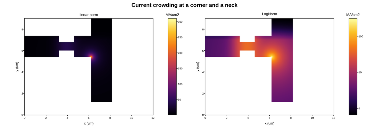
Current density through an on-chip metal interconnect that necks down and turns a corner. Electromigration – metal atoms carried along by the electron wind – scales steeply with current density, so the peak value and where it sits decide how long the wire survives. Design rules are written as a current-density limit, and this is the map they are checked against.

The distribution is extremely skewed. Current crowds into the inside of the corner and the narrow neck while the wide sections carry very little, spanning three or four decades across one structure. Linearly normalised, the whole wire is dark except a couple of pixels, and the gradient that actually drives failure is invisible. LogNorm makes each decade legible.

Current density is a positive magnitude here, which is what admits a log scale; the surrounding dielectric carries no current at all and is nan, so it is left unpainted rather than plotted as a spurious zero the log could not take.

Live figure — pick a tool, then zoom, pan, point-pick or annotate. Nothing is active until a tool is selected.

View this figure’s Vega export ↗ — the raw JSON spec, rendered live by a real Vega engine.

View this figure’s Vega-Lite export ↗ — the raw JSON spec(s), rendered live by a real Vega-Lite engine.

import numpy as np
import polars as pl
import plotpress

x = np.linspace(0.0, 12.0, 380)      # micrometres
y = np.linspace(0.0, 9.0, 300)
X, Y = np.meshgrid(x, y)

# An L-shaped wire: wide arm in, neck at the corner, wide arm out.
horizontal = (Y > 5.4) & (Y < 7.4) & (X < 8.2)
vertical = (X > 6.2) & (X < 8.2) & (Y > 1.2)
neck = (X > 3.2) & (X < 4.6) & (Y > 6.0) & (Y < 6.8)
metal = (horizontal | vertical | neck) & ~((X > 3.2) & (X < 4.6) & ~neck
                                           & (Y > 5.4) & (Y < 7.4))

# Streamlines crowd at the inside corner and through the neck.
corner_r = np.hypot(X - 6.2, Y - 5.4)
density = 1.0 + 26.0 / (corner_r + 0.22) ** 1.7          # inside-corner crowding
density += 34.0 * np.exp(-((X - 3.9) ** 2) / 0.9)        # the neck
density *= np.exp(-np.clip(Y - 7.0, 0.0, None) / 0.5)    # falls across the width
density += 0.6

density = np.where(metal, density, np.nan)

# One row per grid cell -- sorted before the reshape below so the pivot
# back to a grid is correct regardless of row order.
field = pl.DataFrame({
    "x": X.ravel(), "y": Y.ravel(), "density": density.ravel(),
}).sort(["y", "x"])

x_axis = field["x"].unique().sort().to_numpy()
y_axis = field["y"].unique().sort().to_numpy()
density = field["density"].to_numpy().reshape(y_axis.size, x_axis.size)

fig, axes = plotpress.subplots(1, 2, figsize=(12.0, 4.2))
lin = axes[0].pcolormesh(x_axis, y_axis, density, cmap="inferno")
axes[0].set_title("linear norm")
fig.colorbar(lin, ax=axes[0]).set_title("MA/cm2")

log = axes[1].pcolormesh(x_axis, y_axis, density, cmap="inferno", norm=plotpress.LogNorm())
axes[1].set_title("LogNorm")
fig.colorbar(log, ax=axes[1]).set_title("MA/cm2")

for ax in axes:
    ax.set_aspect("equal")
    ax.set_xlabel("x (um)")
    ax.set_ylabel("y (um)")
fig.suptitle("Current crowding at a corner and a neck")
fig.tight_layout()